6 Linear algebra

Some material in this chapter is adapted from notes Hye Young You wrote for the math boot camp for the political science PhD program at Vanderbilt.

Linear algebra is an essential tool for understanding multivariate statistics. My main goal here is for you to get familiar with the basics of vector and matrix notation, and the use of matrices to solve linear systems. You are probably already familiar with matrices, at least informally. The typical data set—each row an observation, each column a variable—is formatted like a matrix.

As with all of our topics, but perhaps to an even greater degree here, we will only cover a light introduction. Linear algebra goes very deep. If you want to learn more, I recommend starting with MIT’s freely available undergraduate course.

6.1 Vectors

A vector is an ordered list of numbers. To denote a vector \mathbf{v} of k elements, we write \mathbf{v} = (v_1, v_2, \ldots, v_k), or sometimes \mathbf{v} = \begin{pmatrix} v_1 \\ v_2 \\ \vdots \\ v_k \end{pmatrix}.

Notice the convention of using a lowercase bold letter to denote a vector. When I write vectors on the whiteboard, I will instead denote them with an arrow, like \vec{v}. We will usually be dealing with vectors of real numbers. To denote the fact that \mathbf{v} is a vector of k real numbers, we write \mathbf{v} \in \mathbb{R}^k.

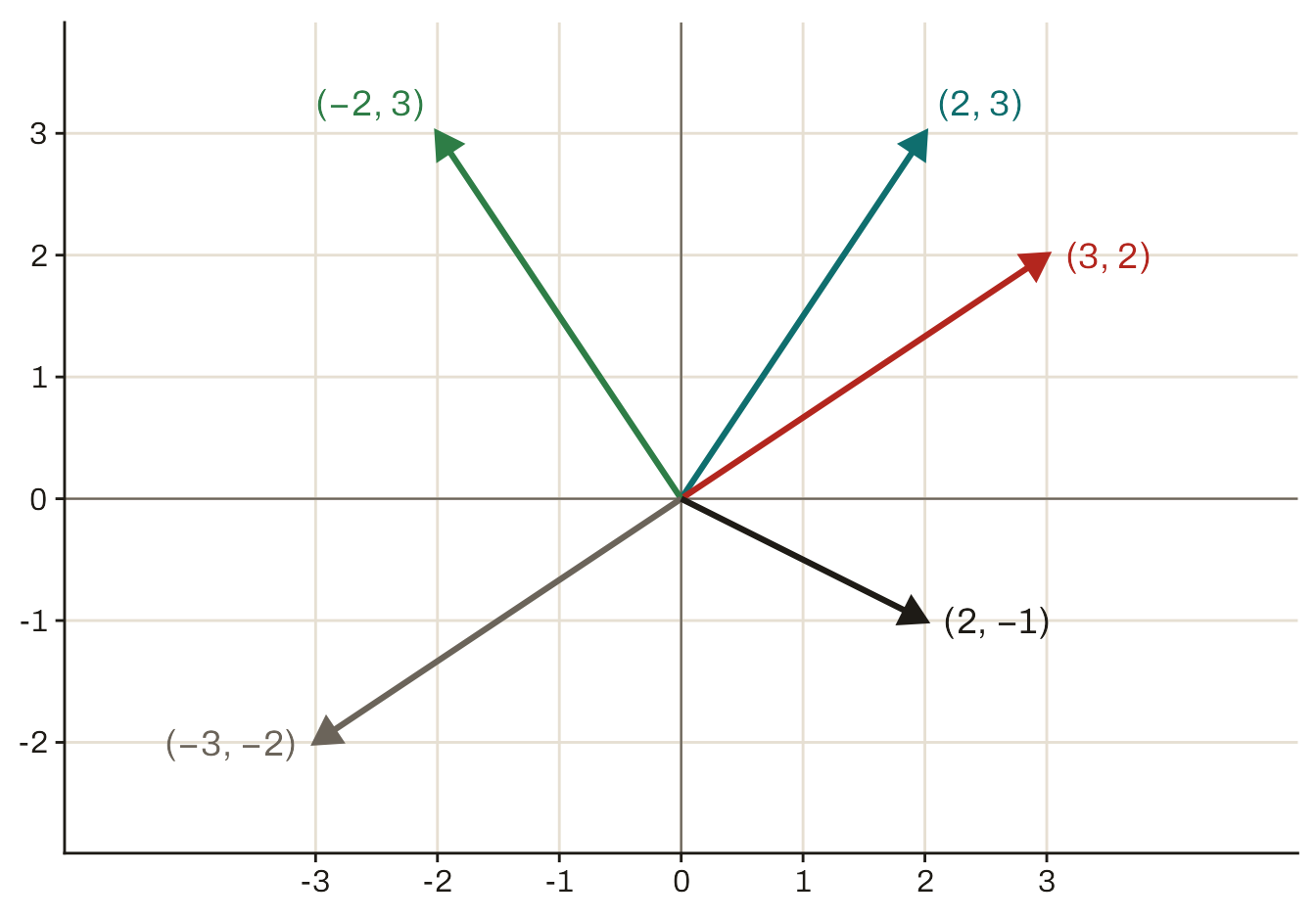
You can think of a vector \mathbf{v} \in \mathbb{R}^k as a point in k-dimensional space. More often, it’s convenient—for reasons we’ll see in just a second—to portray the vector as an arrow pointing from the origin to the given coordinates in k-dimensional space. I personally have a lot of trouble visualizing in more than two dimensions, so I’m going to illustrate all the concepts here with vectors in \mathbb{R}^2.

A vector may seem like a set, but it’s not exactly. In a vector, unlike a set, order matters: the 2-dimensional vectors (2, 3) and (3, 2) are legitimately different, whereas the sets \{2, 3\} and \{3, 2\} are exactly the same.

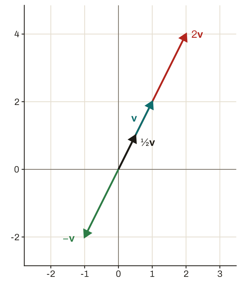
A vector can be multiplied by a scalar c \in \mathbb{R}. Algebraically, this works by just multiplying element-by-element: c \mathbf{v} = \begin{pmatrix} c v_1 \\ c v_2 \\ \vdots \\ c v_k \end{pmatrix}. If c is positive, this looks like an expansion of the vector by a factor of c (or contraction if c < 1). The logic is similar for negative c, except that first the vector is reflected about the origin.

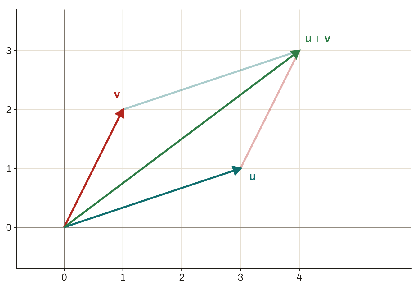
Figure 6.2: Scalar multiplication of the vector \mathbf{v} = (1, 2).

Vector addition also works element-by-element: \mathbf{u} + \mathbf{v} = \begin{pmatrix} u_1 + v_1 \\ u_2 + v_2 \\ \vdots \\ u_k + v_k \end{pmatrix}. This is why it’s convenient to represent vectors as arrows, not just as points in space. If you take the vector \mathbf{u} and start it at the end of \mathbf{v} rather than at the origin, you end up with \mathbf{u} + \mathbf{v}.

Figure 6.3: Addition of the vectors \mathbf{v} = (1, 2) and \mathbf{u} = (3, 1).

A special vector is the zero vector, which contains—you guessed it—all zeroes. We write \mathbf{0}_k to denote the zero vector of length k. When the length of the zero vector is clear from the context, we may just write \mathbf{0}.

The last important vector operation is the dot product. The dot product of \mathbf{u} and \mathbf{v}, written \mathbf{u} \cdot \mathbf{v}, is the sum of the products of the entries: \mathbf{u} \cdot \mathbf{v} = u_1 v_1 + u_2 v_2 + \cdots + u_k v_k = \sum_{m=1}^k u_m v_m. The dot product of two vectors is always a scalar, i.e., a single ordinary number. Since the dot product notation for vectors looks like the same notation as multiplication for scalars, you may be tempted to think that \mathbf{u} \cdot \mathbf{v} will be a vector of element-by-element multiples. Resist the temptation.

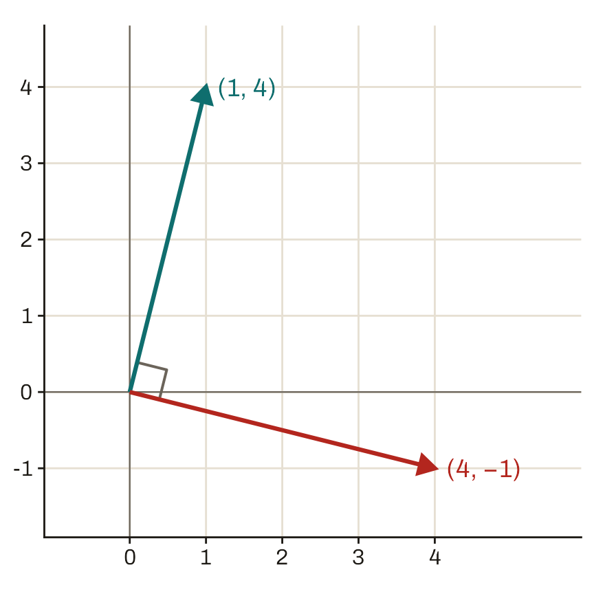
The dot product of two vectors is closely related to the angle between them. Being more specific than that would get us into more geometry, and soon thereafter trigonometry, than I want to do here. So I will just observe that a pair of vectors has a dot product of 0 exactly when they are orthogonal, meaning they are perpendicular to each other.

Figure 6.4: The vectors (1, 4) and (4, -1) have a dot product of 0 and are orthogonal.

Exercise 6.1 (Orthogonal vectors) Find two different vectors that are both orthogonal to \mathbf{v} = (1, 3, 2).

Answer

There are infinitely many answers here, but here are a couple. The vector (3, -1, 0) is orthogonal: \begin{pmatrix} 1 \\ 3 \\ 2 \end{pmatrix} \cdot \begin{pmatrix} 3 \\ -1 \\ 0 \end{pmatrix} = 1 \cdot 3 + 3 \cdot (-1) + 2 \cdot 0 = 0. So is the vector (-3, 1, 0): \begin{pmatrix} 1 \\ 3 \\ 2 \end{pmatrix} \cdot \begin{pmatrix} -3 \\ 1 \\ 0 \end{pmatrix} = 1 \cdot (-3) + 3 \cdot 1 + 2 \cdot 0 = 0. In fact, once we showed that (3, -1, 0) was orthogonal, it turns out that any scalar multiple of it is also orthogonal, as covered in the exercise below.

Exercise 6.2 (Dot product of a scalar multiple) Let \mathbf{u} and \mathbf{v} be vectors of the same length, and let a and b be scalars. Show that a \mathbf{u} \cdot b \mathbf{v} = a b (\mathbf{u} \cdot \mathbf{v}). Using this fact, show that if \mathbf{u} and \mathbf{v} are orthogonal, then so are a \mathbf{u} and b \mathbf{v}.

Answer

Using the definition of scalar multiplication and the dot product, we have \begin{aligned} a \mathbf{u} \cdot b \mathbf{v} &= \begin{pmatrix} a u_1 \\ a u_2 \\ \vdots \\ a u_k \end{pmatrix} \cdot \begin{pmatrix} b v_1 \\ b v_2 \\ \vdots \\ b v_k \end{pmatrix} \\ &= \sum_{m=1}^k (a u_m) (b v_m) \\ &= \sum_{m=1}^k a b u_m v_m \\ &= a b \sum_{m=1}^k u_m v_m \\ &= a b (\mathbf{u} \cdot \mathbf{v}). \end{aligned} If \mathbf{u} and \mathbf{v} are orthogonal, then we have \mathbf{u} \cdot \mathbf{v} = 0. Therefore, a \mathbf{u} \cdot b \mathbf{v} = ab \cdot 0 = 0, so a \mathbf{u} and b \mathbf{v} are orthogonal as well.

6.2 Linear independence

An important concept for regression analysis is the linear independence of a collection of vectors. In essence, to run a regression on a set of variables, you need each column to carry some new information that none of the others already captures. Linear independence formalizes this concept.

Definition 6.1 (Linear independence) A collection of vectors \mathbf{v}_1, \ldots, \mathbf{v}_J is linearly independent if the only solution to c_1 \mathbf{v}_1 + \cdots + c_J \mathbf{v}_J = \mathbf{0} is c_1 = 0, \ldots, c_J = 0. Otherwise, we call the vectors linearly dependent.

As an example, consider the pair of vectors \mathbf{v}_1 = \begin{pmatrix} 1 \\ 0 \end{pmatrix}, \quad \mathbf{v}_2 = \begin{pmatrix} 0 \\ 1 \end{pmatrix}. To check whether they are linearly independent, we need to find every pair of numbers c_1 and c_2 that makes c_1 \mathbf{v}_1 + c_2 \mathbf{v}_2 = \mathbf{0}. Working entry by entry: \begin{aligned} c_1 \mathbf{v}_1 + c_2 \mathbf{v}_2 = \mathbf{0} &\quad \Leftrightarrow \quad \begin{pmatrix} c_1 \cdot 1 + c_2 \cdot 0 \\ c_1 \cdot 0 + c_2 \cdot 1 \end{pmatrix} = \begin{pmatrix} 0 \\ 0 \end{pmatrix} \\ &\quad \Leftrightarrow \quad \begin{pmatrix} c_1 \\ c_2 \end{pmatrix} = \begin{pmatrix} 0 \\ 0 \end{pmatrix}. \end{aligned} The only solution is c_1 = c_2 = 0, so these vectors are linearly independent.

As an example of two linearly dependent vectors, consider \mathbf{v}_1 = \begin{pmatrix} 1 \\ 2 \end{pmatrix}, \quad \mathbf{v}_2 = \begin{pmatrix} 2 \\ 4 \end{pmatrix}. To show that they’re linearly dependent, we just need to find any pair of coefficients to put on them that makes their sum equal (0, 0). Since \mathbf{v}_2 = 2 \mathbf{v}_1, the coefficients c_1 = 2 and c_2 = -1 will work: 2 \mathbf{v}_1 + (-1) \mathbf{v}_2 = \begin{pmatrix} 2 \cdot 1 + (-1) \cdot 2 \\ 2 \cdot 2 + (-1) \cdot 4 \end{pmatrix} = \begin{pmatrix} 2 - 2 \\ 4 - 4 \end{pmatrix} = \begin{pmatrix} 0 \\ 0 \end{pmatrix}.

Some fun facts about linear independence:

If any vector in \mathbf{v}_1, \ldots, \mathbf{v}_J is a linear combination of the others, meaning it can be written as a weighted sum of the others (i.e., \mathbf{v}_j = \sum_{i \neq j} c_i \mathbf{v}_i for some real numbers c_i), then these vectors are linearly dependent.
A collection of J vectors of length k cannot be linearly independent if J > k. In other words, given vectors of length k, the most that can be linearly independent of each other is k.
If any \mathbf{v}_j = \mathbf{0}, then \mathbf{v}_1, \ldots, \mathbf{v}_J are linearly dependent. (Why?)

Exercise 6.3 (Zero vector is always linearly dependent) Explain why a collection of vectors is linearly dependent if any one of them is a zero vector.

Answer

Consider a collection \mathbf{v}_1, \ldots, \mathbf{v}_J where some \mathbf{v}_j = \mathbf{0}. Set the coefficient on \mathbf{v}_j to 1 and every other coefficient to 0: c_1 = 0, \; \ldots, \; c_{j-1} = 0, \quad c_j = 1, \quad c_{j+1} = 0, \; \ldots, \; c_J = 0. Then every term drops out except the j’th one, so c_1 \mathbf{v}_1 + \cdots + c_j \mathbf{v}_j + \cdots + c_J \mathbf{v}_J = \mathbf{v}_j = \mathbf{0}. Because c_j = 1 is not zero, this is a solution other than all zeroes, so the vectors are linearly dependent.

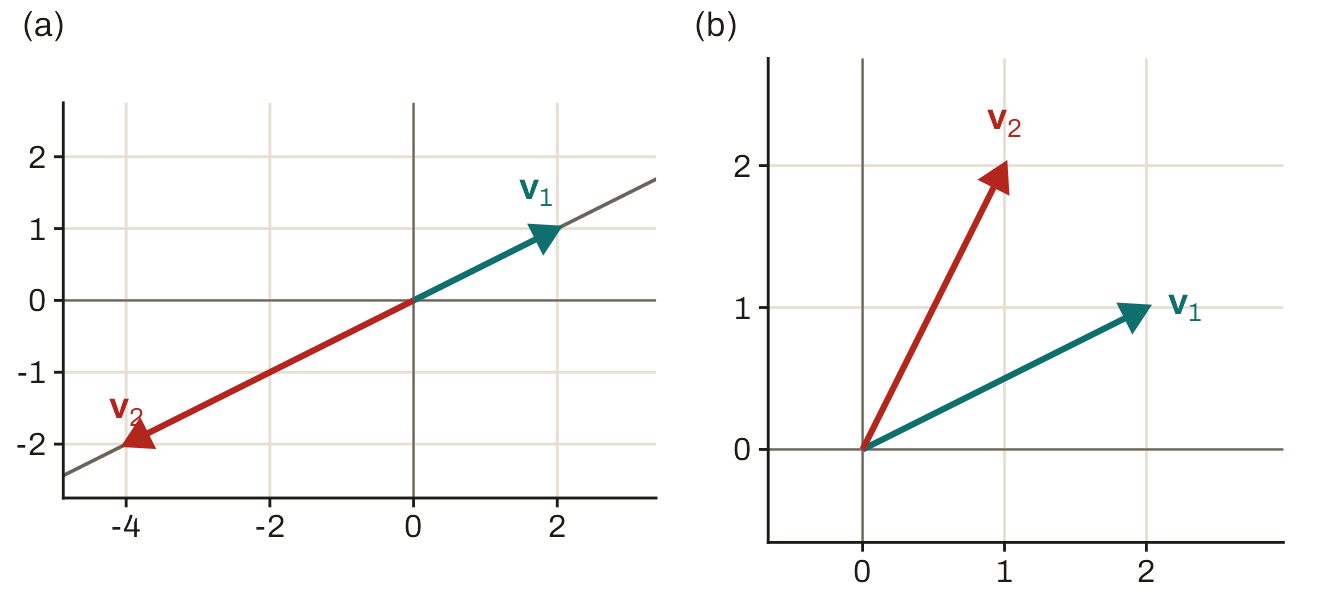
For a collection of two vectors in two-dimensional space, linear dependence has a simple geometric interpretation. The two vectors are linearly dependent exactly when they lie on a common line through the origin, as in panel (a) of Figure 6.5. If the two vectors don’t lie on a common line, as in panel (b), neither one is a scalar multiple of the other, and they are linearly independent.

Figure 6.5: A linearly dependent pair of vectors in \mathbb{R}^2 (a) and a linearly independent pair (b).

Exercise 6.4 (Checking linear independence) Determine whether each of the following collections of vectors is linearly independent.

\mathbf{v}_1 = \begin{pmatrix} 1 \\ 2 \\ 3 \end{pmatrix}, \mathbf{v}_2 = \begin{pmatrix} 2 \\ 4 \\ 6 \end{pmatrix}.
\mathbf{v}_1 = \begin{pmatrix} 1 \\ 2 \\ 3 \end{pmatrix}, \mathbf{v}_2 = \begin{pmatrix} 1 \\ 4 \\ 9 \end{pmatrix}.
\mathbf{v}_1 = \begin{pmatrix} 1 \\ 1 \\ 1 \end{pmatrix}, \mathbf{v}_2 = \begin{pmatrix} 0 \\ 1 \\ 0 \end{pmatrix}, \mathbf{v}_3 = \begin{pmatrix} 0 \\ 0 \\ 1 \end{pmatrix}.
\mathbf{v}_1 = \begin{pmatrix} 1 \\ 0 \\ 0 \end{pmatrix}, \mathbf{v}_2 = \begin{pmatrix} 14 \\ 12 \\ 0 \end{pmatrix}, \mathbf{v}_3 = \begin{pmatrix} 0 \\ -1 \\ 0 \end{pmatrix}.

Answer

Linearly dependent: 2 \mathbf{v}_1 - \mathbf{v}_2 = \mathbf{0}.
Linearly independent: \begin{aligned} & c_1 \mathbf{v}_1 + c_2 \mathbf{v}_2 = \begin{pmatrix} c_1 + c_2 \\ 2 c_1 + 4 c_2 \\ 3 c_1 + 9 c_2 \end{pmatrix} = \mathbf{0} \\ & \quad \Rightarrow \quad c_1 = -c_2 \text{ and } 2 c_2 = 0 \\ & \quad \Rightarrow \quad c_1 = c_2 = 0. \end{aligned}
Linearly independent: c_1 \mathbf{v}_1 + c_2 \mathbf{v}_2 + c_3 \mathbf{v}_3 = \begin{pmatrix} c_1 \\ c_1 + c_2 \\ c_1 + c_3 \end{pmatrix} = \mathbf{0} \quad \Rightarrow \quad c_1 = c_2 = c_3 = 0.
Linearly dependent: 14 \mathbf{v}_1 - \mathbf{v}_2 - 12 \mathbf{v}_3 = \mathbf{0}.

6.3 Concept review

Vector: An ordered array. A vector \mathbf{v} of k elements is written \mathbf{v} = (v_1, v_2, \ldots, v_k). If its elements are real numbers, we write \mathbf{v} \in \mathbb{R}^k.
Zero vector: The vector whose entries are all zeroes. We write \mathbf{0}_k for the zero vector of length k, or just \mathbf{0} when the length is clear from the context.
Dot product: The dot product of \mathbf{u} and \mathbf{v}, written \mathbf{u} \cdot \mathbf{v}, is the sum of the products of the entries: \mathbf{u} \cdot \mathbf{v} = u_1 v_1 + u_2 v_2 + \cdots + u_k v_k.
Scalar: A regular number, which you can think of as a 1-dimensional vector if you want to be pretentious.
Orthogonal: The vectors \mathbf{u} and \mathbf{v} are orthogonal if \mathbf{u} \cdot \mathbf{v} = 0, which is true precisely when they are perpendicular to each other.
Linear independence: The vectors \mathbf{v}_1, \ldots, \mathbf{v}_J are linearly independent if the only solution to c_1 \mathbf{v}_1 + \cdots + c_J \mathbf{v}_J = \mathbf{0} is c_1 = 0, \ldots, c_J = 0. Otherwise, they are linearly dependent.
Linear combination: The vector \mathbf{u} is a linear combination of \mathbf{v}_1, \ldots, \mathbf{v}_J if there are real numbers c_1, \ldots, c_J such that \mathbf{u} = c_1 \mathbf{v}_1 + \cdots + c_J \mathbf{v}_J.

Dot product: The dot product of \mathbf{u} and \mathbf{v}, written \mathbf{u} \cdot \mathbf{v}, is the sum of the products of the entries: \mathbf{u} \cdot \mathbf{v} = u_1 v_1 + u_2 v_2 + \cdots + u_k v_k.
Linear combination: The vector \mathbf{u} is a linear combination of \mathbf{v}_1, \ldots, \mathbf{v}_J if there are real numbers c_1, \ldots, c_J such that \mathbf{u} = c_1 \mathbf{v}_1 + \cdots + c_J \mathbf{v}_J.
Linear independence: The vectors \mathbf{v}_1, \ldots, \mathbf{v}_J are linearly independent if the only solution to c_1 \mathbf{v}_1 + \cdots + c_J \mathbf{v}_J = \mathbf{0} is c_1 = 0, \ldots, c_J = 0. Otherwise, they are linearly dependent.
Orthogonal: The vectors \mathbf{u} and \mathbf{v} are orthogonal if \mathbf{u} \cdot \mathbf{v} = 0, which is true precisely when they are perpendicular to each other.
Scalar: A regular number, which you can think of as a 1-dimensional vector if you want to be pretentious.
Vector: An ordered array. A vector \mathbf{v} of k elements is written \mathbf{v} = (v_1, v_2, \ldots, v_k). If its elements are real numbers, we write \mathbf{v} \in \mathbb{R}^k.
Zero vector: The vector whose entries are all zeroes. We write \mathbf{0}_k for the zero vector of length k, or just \mathbf{0} when the length is clear from the context.