4 Integrals

4.1 Area under the curve

Let’s take a very simple mathematical model of polarized public opinion. Imagine that everyone has an “ideology,” which we’ll represent as a real number between -1 (most liberal) and +1 (most conservative). There are very many people and very many gradations of ideology, so we will represent the distribution of ideology in the public along a continuum.

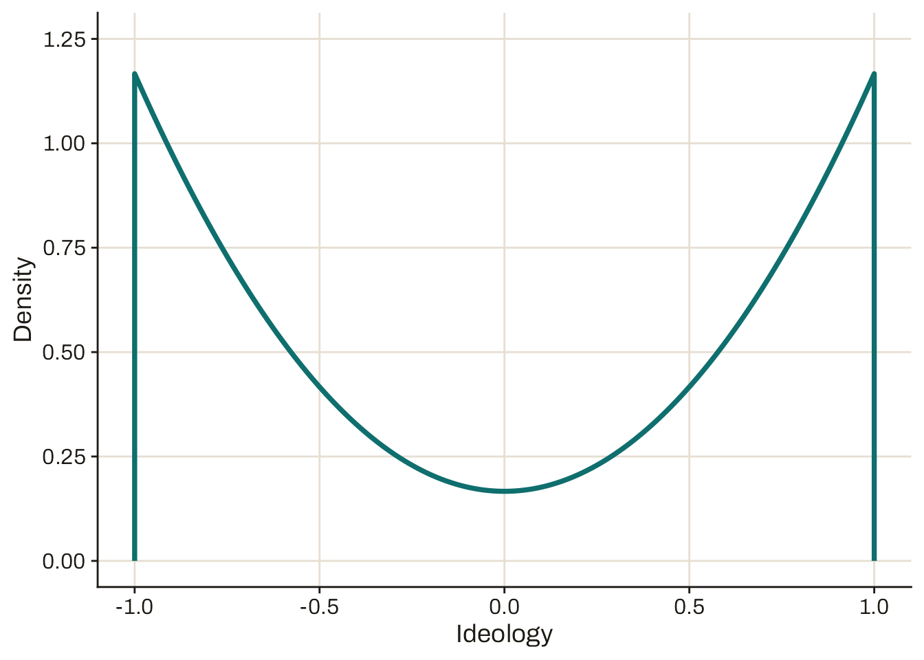
To make this a bit more specific, imagine that the density of ideology has the following bimodal shape.

Figure 4.1: A hypothetical bimodal distribution of ideology.

Suppose we define a center-left person as someone whose ideology lies between -1/2 and 0. If the distribution of preferences looks like Figure 4.1, then what proportion of people are center left? To calculate that, we’d want to calculate the area that falls under the curve between -1/2 and 0, and compare that to the total area under the curve.

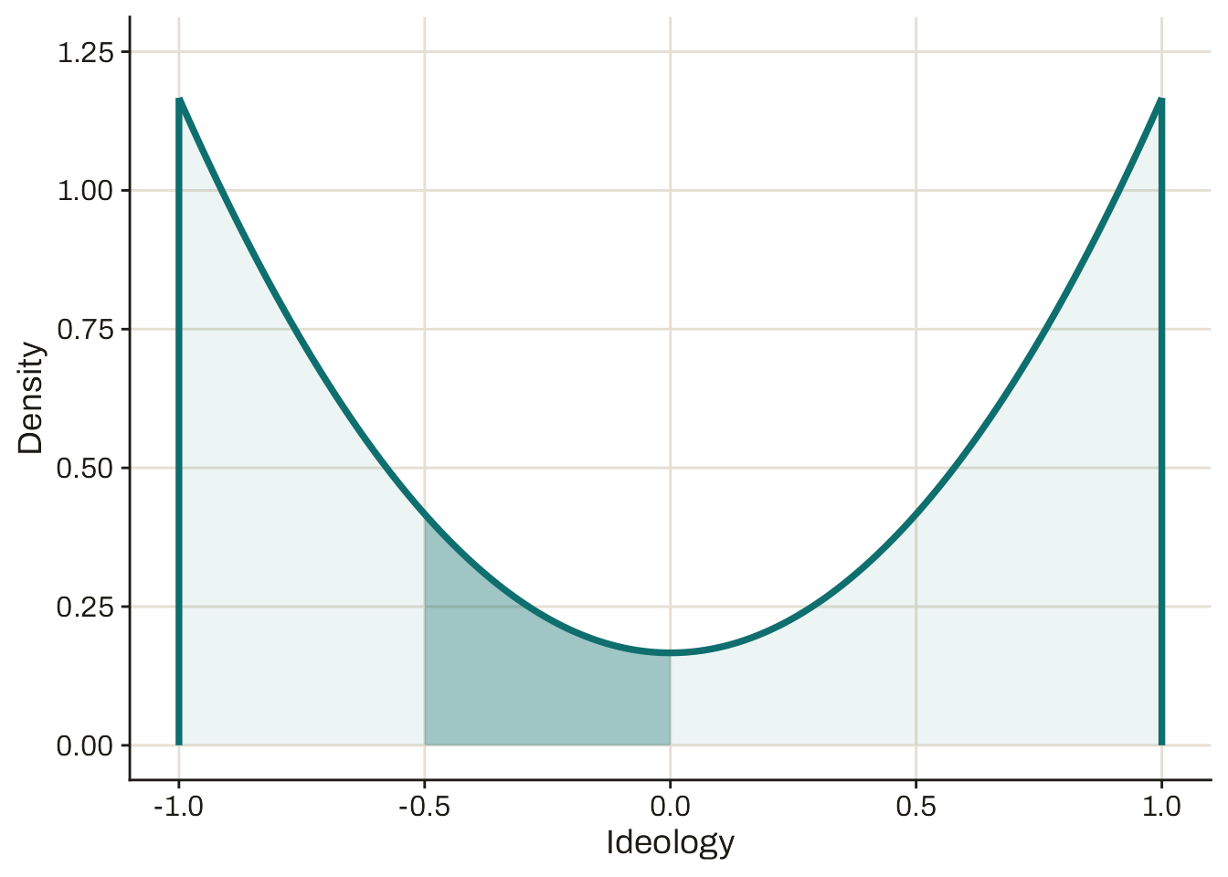
Figure 4.2: The center-left slice of the ideological distribution.

These area calculations are known as integrals. This type of calculation comes up repeatedly in probability and statistics with continuous random variables, so it is important to at least learn the basics. We will cover the bare minimum here, just enough for you to get started. The most important thing to know is a surprising fact—there is a deep connection between derivatives and these area calculations.

4.2 Antiderivatives

It turns out that to calculate the area under a curve given by the function f(x), we will need to find the function whose derivative is equal to f. We call such a function an antiderivative of f.

Definition 4.1 (Antiderivative) Consider functions f : X \to \mathbb{R} and F : X \to \mathbb{R}, where X \subseteq \mathbb{R}. F is an antiderivative of f if F is differentiable and F'(x) = f(x) for all x \in X.

As one example, F(x) = x^2 is an antiderivative of f(x) = 2x. Using the power rule (see Section 3.3.1), we have F'(x) = 2 \cdot x^1 = 2x = f(x).

Exercise 4.1 (Confirming an antiderivative) Define the functions f, F, and G, all mapping \mathbb{R} into \mathbb{R}, by \begin{aligned} f(x) &= 3x^2 + 8x + 7, \\ F(x) &= x^3 + 4x^2 + 7x, \\ G(x) &= x^3 + 4x^2 + 7x + 3. \end{aligned} Confirm that F and G are both antiderivatives of f.

Answer

Using what we know about the derivatives of polynomials (see Exercise 3.8), we have \begin{aligned} F'(x) &= 3x^2 + 4 \cdot 2x^1 + 7 \cdot x^0 \\ &= 3x^2 + 8x + 7 \\ &= f(x); \\ G'(x) &= 3x^2 + 4 \cdot 2x^1 + 7 \cdot x^0 + 0 \\ &= 3x^2 + 8x + 7 \\ &= f(x). \end{aligned}

You saw in Exercise 4.1 that one function may have multiple antiderivatives. This is not specific to the particular function in the example. In fact, if a function has one antiderivative, then it has infinitely many antiderivatives: you can form a new one by shifting the existing one up or down by any constant.

Proposition 4.1 (Multiplicity of antiderivatives) Let F be an antiderivative of f, and let c \in \mathbb{R} be any constant. The function G defined by G(x) = F(x) + c is also an antiderivative of f.

Proof. For all x in the domain, we have \begin{aligned} G'(x) &= \frac{d}{dx} \left[F(x) + c\right] \\ &= F'(x) + \underbrace{\left[\frac{d}{dx} c\right]}_{=0} \\ &= f(x), \end{aligned} so G is an antiderivative of f.

It is relatively easy to find the antiderivative of a polynomial. To see why, let’s start with the antiderivative of a power function, i.e., a function of the form f(x) = x^a. If a \neq -1, then any function of the form F(x) = \frac{1}{a + 1} x^{a+1} + c is an antiderivative. To see why, use the power rule (see Section 3.3.1) and the constant multiple rule (Proposition 3.2): \begin{aligned} F'(x) &= \frac{d}{d x} \left[\frac{1}{a + 1} x^{a + 1} + c\right] \\ &= \frac{1}{a + 1} \cdot \left[\frac{d}{dx} x^{a + 1}\right] + 0 \\ &= \frac{1}{a + 1} \cdot (a + 1) \cdot x^{(a + 1) - 1} \\ &= x^a. \end{aligned}

Remember that a polynomial is a finite sum of power functions, each multiplied by a coefficient. Formally, a polynomial is a function of the form f(x) = c_n x^n + c_{n-1} x^{n-1} + \cdots + c_1 x + c_0 = \sum_{k=0}^n c_k x^k, where each c_k is a constant real number. Using the antiderivative of a power function, we have that any function of the form F(x) = \frac{c_n}{n + 1} x^{n+1} + \frac{c_{n-1}}{n} x^n + \cdots + \frac{c_1}{2} x^2 + c_0 x + c = \sum_{k=0}^n \frac{c_k}{k + 1} x^{k + 1} + c is an antiderivative of f.

Exercise 4.2 (Antiderivatives of polynomials) Find an antiderivative of each polynomial listed here.

f(x) = (x + 2) (x - 2).
f(x) = 40 x^{39} - 10 x^{17} + 27.
General constant function: f(x) = \alpha, where \alpha is a constant.
General linear function: f(x) = \alpha + \beta x, where \alpha and \beta are constants.
General quadratic function: f(x) = \alpha + \beta x + \gamma x^2, where \alpha, \beta, and \gamma are constants.

Answer

We have f(x) = x^2 - 2 x + 2 x - 4 = x^2 - 4, so any function of the form F(x) = \frac{x^3}{3} - 4 x + c is an antiderivative of f.
Any function of the form F(x) = x^{40} - \frac{10 x^{18}}{18} + 27 x + c is an antiderivative of f.
Any function of the form F(x) = \alpha x + c is an antiderivative of f.
Any function of the form F(x) = \alpha x + \frac{\beta x^2}{2} + c is an antiderivative of f.
Any function of the form F(x) = \alpha x + \frac{\beta x^2}{2} + \frac{\gamma x^3}{3} + c is an antiderivative of f.

Exercise 4.3 (Antiderivative of 1/x) Why did I need to impose the assumption that a \neq -1 when claiming that F(x) = \frac{1}{a + 1} x^{a + 1} + c is an antiderivative of f(x) = x^a? What in fact is the form of the antiderivative of f(x) = x^{-1} for x \in (0, \infty)?

Answer

We need a \neq -1 because otherwise a + 1 = 0 and thus \frac{1}{a + 1} is undefined, making the ostensible expression for the antiderivative undefined as well.

Remember that the natural logarithm, \log(x), is defined on the domain (0, \infty) and has a derivative of \frac{1}{x}. Because \frac{1}{x} = x^{-1}, we have that any function of the form F(x) = \log(x) + c is an antiderivative of f(x) = x^{-1} on (0, \infty).

4.3 Calculating integrals

4.3.1 The second fundamental theorem

Usually I like to lead you through the logic behind a mathematical result before telling you the result. But this result is sufficiently important for day-to-day mathematical life, and the logic behind it is sufficiently intricate, that I’m going to just start with the headline finding.

The second fundamental theorem of calculus states that we can calculate an integral by taking the difference between antiderivatives.

Theorem 4.1 (Second fundamental theorem of calculus) Let the integrand f : X \to \mathbb{R} be continuous, where X \subseteq \mathbb{R}, and let F : X \to \mathbb{R} be an antiderivative of f. For any [a, b] \subseteq X, we have \int_a^b f(x) \, dx = F(b) - F(a).

A lot goes into understanding why this theorem “works,” so I am going to put that off for Section 4.3.2 below. Before that, let’s go through a couple of examples where we can calculate the area separately with normal geometric techniques, and confirm that Theorem 4.1 gives us the same answer.

Let’s start by calculating the area under a constant function, f(x) = \alpha, between a and b. As you can see in the illustration below, this amounts to computing the area of a rectangle.

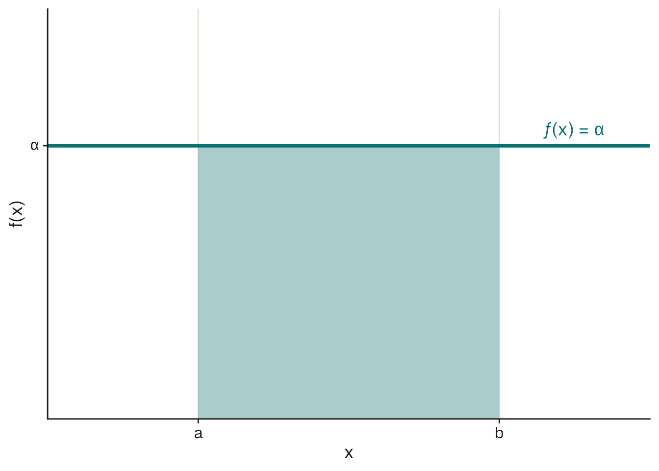
Figure 4.3: Area under a constant function.

The width of this rectangle is b - a and its height is \alpha, so the area under the curve is \alpha (b - a). Let’s see if the second fundamental theorem gives us the same answer. Our function is f(x) = \alpha, so the function F(x) = \alpha x is an antiderivative. The second fundamental theorem then gives us \begin{aligned} \int_a^b f(x) \, dx = F(b) - F(a) = \alpha b - \alpha a = \alpha (b - a), \end{aligned} the same as our geometric area calculation. So far, so good!

Before moving on to another example, I want to take a second to illustrate why it doesn’t matter which antiderivative of f(x) we use in the calculation. Above I used F(x) = \alpha x, but in fact any function of the form F(x) = \alpha x + c is an antiderivative of the constant function f(x) = \alpha. But when we plug in another such function, the c’s cancel out and we get the same answer: F(b) - F(a) = [\alpha b + c] - [\alpha a + c] = \alpha (b - a). This remains true even when calculating integrals of other functions. So when you have to do such a calculation, just pick whichever antiderivative is easiest (almost always by setting c = 0).

Now let’s think about calculating the area under the line f(x) = \beta (x - a), from where it crosses the x-axis at x = a up to some other point x = b. As you can see in the illustration below, this amounts to computing the area of a triangle.

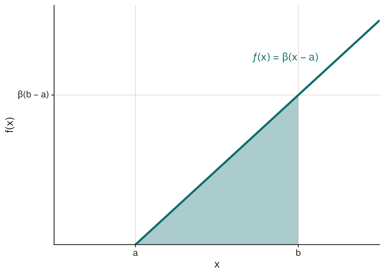
Figure 4.4: Area under a linear function, starting from where it crosses the x-axis.

The triangle has a width of b - a and a height of \beta (b - a), so its area is \frac{1}{2} \cdot (b - a) \cdot [\beta (b - a)] = \frac{\beta}{2} (b - a)^2. Let’s again see if Theorem 4.1 gives us the same answer. Our function is f(x) = \beta (x - a) = \beta x - \beta a, so F(x) = \frac{\beta}{2} x^2 - \beta a x is an antiderivative. The second fundamental theorem then gives us \begin{aligned} \int_a^b f(x) \, dx &= F(b) - F(a) \\ &= \left[\frac{\beta}{2} b^2 - \beta a b\right] - \left[\frac{\beta}{2} a^2 - \beta a^2\right] \\ &= \frac{\beta}{2} b^2 - \beta a b - \frac{\beta}{2} a^2 + \beta a^2 \\ &= \frac{\beta}{2} b^2 - \beta a b + \frac{\beta}{2} a^2 \\ &= \frac{\beta}{2} \left[b^2 - 2 a b + a^2\right] \\ &= \frac{\beta}{2} (b - a)^2. \end{aligned} The algebra to get there was a bit uglier than with the rectangle, but ultimately once again the calculus gives us the same answer as the geometry.

Exercise 4.4 (Back to the motivating example) Let’s go back to the example illustrated in Figure 4.2, where we want to calculate the proportion of people who are “center left.” The function plotted there is the polynomial f(x) = x^2 + \frac{1}{6}.

Identify an antiderivative of f.
Confirm that the total area under the curve is 1.
Find the proportion of people who are center-left by calculating \int_{-1/2}^0 f(x) \, dx.

Answer

One antiderivative is F(x) = \frac{x^3}{3} + \frac{x}{6}.
To calculate the total area under the curve, we take the integral \begin{aligned} \int_{-1}^1 f(x) \, dx &= F(1) - F(-1) \\ &= \left[\frac{1}{3} + \frac{1}{6}\right] - \left[\frac{-1}{3} + \frac{-1}{6}\right] \\ &= 2 \left[\frac{1}{3} + \frac{1}{6}\right] \\ &= 2 \cdot \frac{3}{6} \\ &= 1. \end{aligned}
The proportion of people who are center-left is \begin{aligned} \int_{-1/2}^0 f(x) \, dx &= F(0) - F(-1/2) \\ &= \left[\frac{0}{3} + \frac{0}{6}\right] - \left[\frac{-1/8}{3} + \frac{-1/2}{6}\right] \\ &= \frac{1}{24} + \frac{1}{12} \\ &= \frac{3}{24} \\ &= \frac{1}{8}. \end{aligned}

One last thing to clean up before we move into explanations and properties. If you are pedantic like me, you might be wondering, “What if the function doesn’t have an antiderivative? Then does the integral even exist?” It turns out, via the first fundamental theorem of calculus, that every continuous function whose domain is an interval has an antiderivative. Therefore, for any continuous f : [a, b] \to \mathbb{R}, the integral \int_a^b f(x) \, dx is well-defined.

4.3.2 Explaining the second fundamental theorem

TBA.

4.4 Properties of the integral

Constant multiple rule: \int_a^b c f(x) \, dx = c \int_a^b f(x) \, dx.

Sum rule: \int_a^b [f(x) + g(x)] \, dx = \int_a^b f(x) \, dx + \int_a^b g(x) \, dx.

Addition across subdomains: if a \leq c \leq b, \int_a^b f(x) \, dx = \int_a^c f(x) \, dx + \int_c^b f(x) \, dx.

Wrong way limits: \int_a^b f(x) \, dx = -\int_b^a f(x) \, dx.

Comparing integrals: if f(x) \geq (>) g(x) for all x \in (a, b), then \int_a^b f(x) \, dx \geq (>) \int_a^b g(x) \, dx.

Corollary to the comparison: if f(x) is (strictly) positive on (a, b), then so is \int_a^b f(x) \, dx.

Full statements and explanations TBA.

4.5 The chain rule in reverse: Integration by substitution

It would be nice to only ever have to take integrals of polynomials, but sadly that’s not the world we live in. Sometimes you have to integrate functions where there’s no surefire algorithm to obtain an antiderivative. There are many, many methods of integrating these functions. We will just look at the technique that, in my experience, comes up most frequently—integration by substitution.

For example, think about computing the integral \int_0^1 \frac{4x}{x^2 + 7} \, dx. How are we supposed to have any hope of computing this integral? It’s actually not nearly as bad as it looks. It turns out that we can define a new variable u as u = x^2 + 7 and end up with \int_0^1 \frac{4x}{x^2 + 7} \, dx = 2 \int_7^8 \frac{1}{u} \, du = 2 [\log 8 - \log 7]. This move is justified by integration by substitution, which in turn is justified by the chain rule for derivatives (Proposition 3.6). I’ll state the general result, then show how we get to the integral in the example.

Proposition 4.2 (Integration by substitution) Let Y \subseteq \mathbb{R} be an interval. If g : [a, b] \to Y is continuously differentiable (i.e., g is differentiable, and its derivative g' is itself a continuous function) and f : Y \to \mathbb{R} is continuous, then \int_a^b f(g(x)) g'(x) \, dx = \int_{g(a)}^{g(b)} f(u) \, du.

Proof. Assume g : [a, b] \to Y is continuously differentiable and f : Y \to \mathbb{R} is continuous, and let F be an antiderivative of f. Let h : [a, b] \to \mathbb{R} be defined by h(x) = f(g(x)) g'(x), and let H : [a, b] \to \mathbb{R} be defined by H(x) = F(g(x)). By the chain rule, H is an antiderivative of h: H'(x) = F'(g(x)) \cdot g'(x) = f(g(x)) g'(x) = h(x). Therefore, by the second fundamental theorem of calculus, \begin{aligned} \int_a^b f(g(x)) g'(x) \, dx &= \int_a^b h(x) \, dx \\ &= H(b) - H(a) \\ &= F(g(b)) - F(g(a)). \end{aligned} Applying the second fundamental theorem again in the other direction, we have F(g(b)) - F(g(a)) = \int_{g(a)}^{g(b)} f(u) \, du. We conclude that \int_a^b f(g(x)) g'(x) \, dx = \int_{g(a)}^{g(b)} f(u) \, du.

To see this method in action, let’s return to the problem of calculating \int_0^1 \frac{4x}{x^2 + 7} \, dx. The really inconvenient thing in this integral is the x^2 + 7 in the denominator, so let’s see if we can simplify the integral with the substitution g(x) = x^2 + 7. The derivative of the substitution is g'(x) = 2x. To apply the rule, we need to isolate the substitution and its derivative: \begin{aligned} \int_0^1 \frac{4x}{x^2 + 7} \, dx &= \int_0^1 \left[\frac{2}{x^2 + 7} \cdot (2x)\right] \, dx \\ &= \int_0^1 \left[\underbrace{\frac{2}{g(x)}}_{f(u) = 2/u} \cdot g'(x)\right] \, dx \\ &= \int_{g(0)}^{g(1)} \frac{2}{u} \, du \\ &= \int_{0^2 + 7}^{1^2 + 7} \frac{2}{u} \, du \\ &= 2 \int_7^8 \frac{1}{u} \, du \\ % &= 2 \left[ \log u \right]_{u=7}^8 \\ &= 2 [\log 8 - \log 7]. \end{aligned}

A more direct way to solve the integral would be to observe that 2 \log(x^2 + 7) is an antiderivative of the original integrand: \begin{aligned} \frac{d}{dx} \left[2 \log(x^2 + 7)\right] &= 2 \frac{d}{dx} \log(x^2 + 7) \\ &= 2 \cdot \frac{1}{x^2 + 7} \cdot \frac{d}{dx} [x^2 + 7] \\ &= 2 \cdot \frac{1}{x^2 + 7} \cdot (2x) \\ &= \frac{4x}{x^2 + 7}. \end{aligned} The second fundamental theorem then ultimately yields the same answer: \int_0^1 \frac{4x}{x^2 + 7} \, dx = \left[2 \log(x^2 + 7)\right]_{x=0}^1 = 2 [\log 8 - \log 7]. The moral of the story here—if you can look at the integrand and figure out its antiderivative, you of course remain free to calculate the integral that way. But if you’re stuck, it can be helpful to try different substitutions to see if any of them yield an integral that you can ultimately take!

Exercise 4.5 (A pretty normal integral) Given any d > 0, use the substitution g(x) = x^2 / 2 to calculate \int_{-d}^{d} x e^{-x^2 / 2} \, dx.

Answer

We have g'(x) = \frac{1}{2} \cdot 2x = x, so integration by substitution gives us \begin{aligned} \int_{-d}^{d} x e^{-x^2 / 2} \, dx &= \int_{-d}^{d} e^{-g(x)} g'(x) \, dx \\ &= \int_{g(-d)}^{g(d)} e^{-u} \, du. \end{aligned} Because g(-d) = g(d) = \frac{d^2}{2}, the second fundamental theorem gives us \int_{g(-d)}^{g(d)} e^{-u} \, du = \left[- e^{-u} \right]_{u=d^2/2}^{d^2/2} = (-e^{-d^2/2}) - (-e^{-d^2/2}) = 0.

Exercise 4.6 (Shifting the domain by a constant) Let f : \mathbb{R} \to \mathbb{R} be a continuous function, and let c \in \mathbb{R} be a constant. Using integration by substitution, show that \int_a^b f(x + c) \, dx = \int_{a + c}^{b + c} f(u) \, du.

Answer

Define g(x) = x + c. The derivative of the substitution is g'(x) = 1, so integration by substitution gives us \begin{aligned} \int_a^b f(x + c) \, dx &= \int_a^b f(g(x)) g'(x) \, dx \\ &= \int_{g(a)}^{g(b)} f(u) \, du \\ &= \int_{a + c}^{b + c} f(u) \, du. \end{aligned}

Exercise 4.7 (The kind of normal integral you’d expect) Let \mu \in \mathbb{R} and d > 0 be constant. Show that \frac{\int_{\mu - d}^{\mu + d} x e^{-(x - \mu)^2 / 2} \, dx}{\int_{\mu - d}^{\mu + d} e^{-(x - \mu)^2 / 2} \, dx} = \mu.

Answer

Via Exercise 4.6, use the substitution g(x) = x - \mu to simplify both integrals: \frac{\int_{\mu - d}^{\mu + d} x e^{-(x - \mu)^2 / 2} \, dx}{\int_{\mu - d}^{\mu + d} e^{-(x - \mu)^2 / 2} \, dx} = \frac{\int_{-d}^d (v + \mu) e^{-v^2 / 2} \, dv}{\int_{-d}^d e^{-v^2 / 2} \, dv}. Use the addition and constant multiplication properties of the integral to simplify the numerator: \begin{aligned} \int_{-d}^d (v + \mu) e^{-v^2 / 2} \, dv &= \int_{-d}^d v e^{-v^2 / 2} \, dv + \int_{-d}^d \mu e^{-v^2 / 2} \, dv \\ &= \int_{-d}^d v e^{-v^2 / 2} \, dv + \mu \int_{-d}^d e^{-v^2 / 2} \, dv. \end{aligned} We saw in Exercise 4.5 that the first term in this sum equals 0. Therefore, we conclude that \frac{\int_{-d}^d (v + \mu) e^{-v^2 / 2} \, dv}{\int_{-d}^d e^{-v^2 / 2} \, dv} = \frac{\mu \int_{-d}^d e^{-v^2 / 2} \, dv}{\int_{-d}^d e^{-v^2 / 2} \, dv} = \mu, as claimed.

4.6 Concept review

Integral: The integral of f between a and b, denoted \int_a^b f(x) dx, is the signed area between the value of f and the x-axis between x = a and x = b. (By “signed” area, I mean that the value is negative when f(x) < 0.)
Antiderivative: A differentiable function F(x) is an antiderivative of f(x) if F'(x) = f(x) for all x.
Second fundamental theorem of calculus: If F is an antiderivative of a continuous function f, then \int_a^b f(x) dx = F(b) - F(a).
Integrand: The function being integrated, i.e., the f(x) in the integral \int_a^b f(x) dx.
Integration by substitution: The reverse of the chain rule for integrals: \int_a^b f(g(x)) g'(x) dx = \int_{g(a)}^{g(b)} f(u) du.

Antiderivative: A differentiable function F(x) is an antiderivative of f(x) if F'(x) = f(x) for all x.
Integral: The integral of f between a and b, denoted \int_a^b f(x) dx, is the signed area between the value of f and the x-axis between x = a and x = b. (By “signed” area, I mean that the value is negative when f(x) < 0.)
Integrand: The function being integrated, i.e., the f(x) in the integral \int_a^b f(x) dx.
Integration by substitution: The reverse of the chain rule for integrals: \int_a^b f(g(x)) g'(x) dx = \int_{g(a)}^{g(b)} f(u) du.
Second fundamental theorem of calculus: If F is an antiderivative of a continuous function f, then \int_a^b f(x) dx = F(b) - F(a).