2 Limits and Continuity – Mathematical Foundations of Political Analysis

2.1 Introduction

We saw in our discussion of set theory (Chapter 1) that math is not just for numbers. That said, you will be working with numbers a lot in your careers as political scientists, especially when using statistics. So to get you where you need to go with statistical analysis, we will be narrowing our focus to the real numbers, \mathbb{R}, and to functions that map from and to (subsets of) the real numbers.

The mathematical foundations of the most important statistical techniques involve the two core operations in calculus, derivatives and integrals. Those operations in turn depend on limits and continuity of functions, the core topics of this chapter.

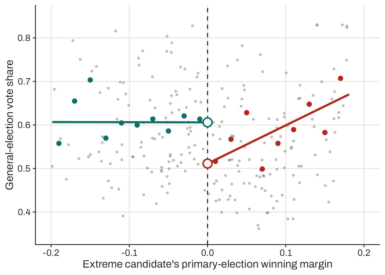
To illustrate the key ideas before we dig into the math, take a look at Figure 2.1, taken from Hall (2015), a study of the effects of ideological extremism on candidates’ eventual success in US House races.

Figure 2.1: Illustration of the main result from Hall (2015), adapted from his Figure 2.

Each of the small points in the graph represents a House race where the top two primary candidates can be sorted into an “extremist” and a “moderate” based on standard estimates of candidate ideology. The x-axis represents the extremist’s margin over the moderate in the primary, and the y-axis represents their party’s vote share in the general election. The left half of the graph therefore represents races where the moderate won the primary and ended up running in the general election, while the right half represents those where the extremist did so. The larger points represent average y values for nearby x values, and the lines are linear trends in general-election outcomes for moderate candidates (left) and for extreme ones (right).

This graph is a substantively important piece of evidence in the ongoing debate in American politics about whether moderation is electorally beneficial. Conveniently for our purposes, it also illustrates the two key concepts we will take on in this section of the course. First, there is the limit of each trend line as it approaches 0. We don’t observe any primaries in which a moderate, or an extremist, wins by exactly 0 votes. But if we project forward—from the average among moderates who win by about 10%, to those who win by about 1%, to those who win by about 0.1%, and so on and so on—the line points to an expected general election vote share of about 61% for our hypothetical moderate who ties the primary and wins by a literal coin flip. Performing the same exercise from the other direction for a hypothetical extremist who wins a tied primary, our limiting projection for the general election is about 52%.

We also see continuity—or, more precisely, a lack of continuity around the threshold between a moderate and an extreme candidate winning the primary. Traveling from left to right across the graph, going from a moderate barely winning to an extremist barely winning, the projected vote share in the general election suddenly “jumps” down by about 9 percentage points. The discontinuity here is statistical evidence for the idea that moderation increases a candidate’s appeal to a general electorate, as you’ll learn in the stats sequence when you cover regression discontinuity designs.

We won’t be going further into the statistical implications of limits and continuity here. We’ll just look at the mathematics behind these ideas, both because they are important in their own right and because they form important building blocks for calculus.

2.2 Limits of functions

2.2.1 Definition

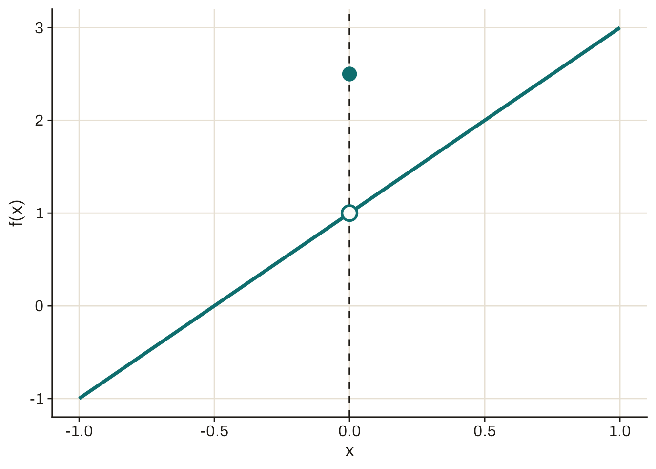
Think about the function f : [-1, 1] \to \mathbb{R} depicted below in Figure 2.2. At every point in the domain besides x = 0, we have f(x) = 1 + 2x. At x = 0, the value of the function “jumps” up to 2.5.

Figure 2.2: A function that “jumps” at a particular point.

Reading and writing cases notation

You might be wondering how we would write the “formula” for a function like the one depicted in Figure 2.2. There are many ways to do so, but I tend to prefer “cases” notation like the following: f(x) = \begin{cases} 1 + 2 x & \text{if $x \neq 0$}, \\ 2.5 & \text{if $x = 0$}. \end{cases} \tag{2.1}

If the formula for a function differs across pieces of its domain, it is convenient to use the cases notation with a curly brace as in Equation 2.1. A cases-notation definition of a function g : A \to B would look something like the following: g(x) = \begin{cases} \text{formula 1} & \text{if $x$ satisfies condition 1}, \\ \text{formula 2} & \text{if $x$ satisfies condition 2}, \\ \vdots \\ \text{formula n} & \text{if $x$ satisfies condition n}. \end{cases} This is a valid way to define g as long as every domain point x \in A satisfies one, and only one of the listed conditions. In other words, the listed conditions must be mutually exclusive (can’t satisfy more than one) and mutually exhaustive (every domain point satisfies at least one). Looking back up at Equation 2.1, these conditions hold for the domain A = [-1, 1]: the first line covers x \in [-1, 0), the second line covers x = 0, and the first line again covers x \in (0, 1].

If we get really close to x = 0 on the domain but not quite there, the value of the function gets really close to 1. This is true no matter how close we get, as long as we don’t go all the way to x = 0 itself. In this sense, we would say the limit of the function as x approaches 0 is equal to 1. In mathematical notation, we would write \lim_{x \to 0} f(x) = 1.

Definition 2.1 (Limit of a function, informal) Consider a function f : X \to Y, where X \subseteq \mathbb{R} and Y \subseteq \mathbb{R}. Let c be a point in the domain of f, i.e., c \in X. We say that a number y is the limit of f(x) as x approaches c, denoted \lim_{x \to c} f(x) = y, if f(x) is very close to y whenever x is very close to (but not exactly equal to) c.

To see how this definition operates in practice, let’s again think about the “jump”-y function pictured in Figure 2.2. Because we are interested in how the function behaves when x is close to 0, we will use the value 0 in place of the arbitrary constant c from the definition. We want to validate that if x is very close to c = 0, though not necessarily equal to it, then the function value f(x) is very close to 1. To convince yourself that this is the case, you can think of smaller and smaller windows of x around c = 0:

Consider x within 0.1 of c = 0 but not equal to it, i.e., x \in (-0.1, 0) \cup (0, 0.1). For all values of x in this range, we have 0.8 < f(x) < 1.2.
Now consider a narrower range, x \in (-0.01, 0) \cup (0, 0.01). For all values of x in this range, we have 0.98 < f(x) < 1.02.
Go another order of magnitude smaller, and think about x \in (-0.001, 0) \cup (0, 0.001). For all values of x in this range, we have 0.998 < f(x) < 1.002.

Hopefully, you see that as we shrink the band around c = 0 to become narrower and narrower, the band of values of f(x) is also shrinking to be narrower and narrower around f(x) = 1. If you kept repeating this process indefinitely for smaller and smaller bands around c = 0, you would see that the band of f(x) values indefinitely became smaller and smaller as well.

You may wonder: where does it stop? How “close” is close enough? How small of a band around c do I need to draw to be sure of the value of the limit? For example, by going down to c \pm 0.001 in the example above, we were able to narrow down to 0.998 < f(x) < 1.002, but how do we know that the limit is exactly 1?

These are hard questions that stumped philosophers and mathematicians at least as far back as Zeno and his paradoxes, if not even earlier. Only in the 1800s did mathematicians finally settle on formal definitions that answer these questions satisfactorily (Gowers 2008, 122–26). Unfortunately, those formal definitions are pretty tricky to work with, which is why I’ve shunted them off to optional material in Section 2.5. Fortunately, for most day-to-day applications of limits—including, importantly, the derivatives you’ll be taking once we move into calculus—you don’t need the full definition and can just rely on the properties outlined below.

Exercise 2.1 (Cases notation and the limit of a function) Consider the function f : [0, 4] \to \mathbb{R} defined by f(x) = \begin{cases} x^2 - 1 & \text{if $0 \leq x < 2,$} \\ 1 & \text{if $x = 2,$} \\ -2x + 7 & \text{if $2 < x \leq 4.$} \end{cases} Graph this function. Eyeball the graph to get an idea of the limit of f(x) as x approaches 2. Then use logic similar to the example above to convince yourself further that your chosen value is indeed the limit.

Answer

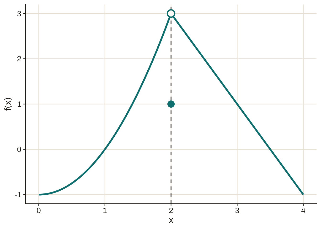
From the graph it looks like \lim_{x \to 2} f(x) = 3. Similar to the example from the text, let’s look at increasingly narrow windows around c = 2, and see if the range of f(x) values gets closer and closer to 3.

Let’s consider values of x within 0.1 of c = 2 without reaching it exactly, i.e., x \in (1.9, 2) \cup (2, 2.1). On the left side, for x \in (1.9, 2), we have 1.9^2 - 1 = 2.61 < f(x) < 3 = 2^2 - 1. On the right side, for x \in (2, 2.1), we have -2 \cdot 2 + 7 = 3 > f(x) > 2.8 = -2 \cdot 2.1 + 7. Altogether, then, we have 2.61 < f(x) < 3 throughout this range.
Going even closer, let’s examine x \in (1.99, 2) \cup (2, 2.01). On the left side, we have 1.99^2 - 1 = 2.9601 < f(x) < 3 = 2^2 - 1. On the right side, we have -2 \cdot 2 + 7 = 3 > f(x) > 2.98 = -2 \cdot 2.01 + 7. So we have 2.9601 < f(x) < 3 throughout this range.
Zooming in by one more order of magnitude, look at x \in (1.999, 2) \cup (2, 2.001). On the left side, 1.999^2 - 1 = 2.996001 < f(x) < 3 = 2^2 - 1. On the right side, -2 \cdot 2 + 7 = 3 > f(x) > 2.998 = -2 \cdot 2.001 + 7. So we have 2.996001 < f(x) < 3 throughout this range.

If we were to keep repeating this process for smaller and smaller bands around c = 2, we would keep ending up with 2.99\cdots < f(x) < 3, with the left-hand number getting ever closer and closer to 3. Therefore, we conclude that \lim_{x \to 2} f(x) = 3.

2.2.2 Properties of limits

Most of the time, when you need to calculate a limit, you’ll rely on a few simple rules instead of making arguments that go straight back to the definition.

We’ll begin with a couple of statements that may seem obvious, but which give us an important toehold to start using the other properties below. Both of these statements can be proved to be true using the formal definition of a limit (Definition 2.6 in the optional section at the end of this chapter), but we’ll just take them as given for our purposes. The first is that if a function f(x) equals the same constant at all values close to c, then its limit as x approaches c is that same constant.

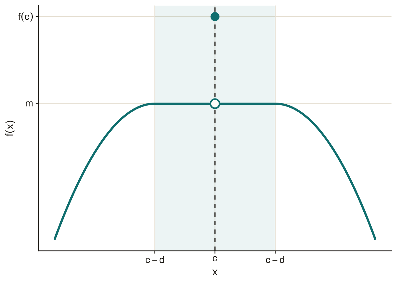
Proposition 2.1 (Limit of a locally constant function) Consider a function f : X \to Y, where X \subseteq \mathbb{R} and Y \subseteq \mathbb{R}. Let c be a point in the domain of f, i.e., c \in X. If there is a positive number d > 0 and a constant (positive, negative, or zero) m \in \mathbb{R} such that f(x) = m \quad \text{for all } x \in (c - d, c) \cup (c, c + d), then \lim_{x \to c} f(x) = m.

In other words, if f(x) equals the same constant m at every value within d units of c (other than, perhaps, c itself) then the limit there must also equal m. Figure 2.3 illustrates a function where this rule would apply.

Figure 2.3: The limit of a locally constant function.

Our other building block is a similar proposition, but this time about the limit of a function where f(x) = x at all values close to c.

Proposition 2.2 (Limit of a local identity function) Consider a function f : X \to Y, where X \subseteq \mathbb{R} and Y \subseteq \mathbb{R}. Let c be a point in the domain of f, i.e., c \in X. If there is a positive number d > 0 such that f(x) = x \quad \text{for all } x \in (c - d, c) \cup (c, c + d), then \lim_{x \to c} f(x) = c.

So if the function overlaps with the 45-degree line for a certain radius around x = c, then its limit as x approaches c is exactly c. Figure 2.4 illustrates this property.

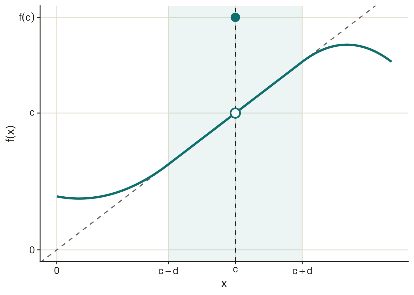
Figure 2.4: The limit of a function that locally coincides with the 45-degree line.

It is not surprising that the limit of a constant function is the constant (Proposition 2.1) or that \lim_{x \to c} x = c (Proposition 2.2). But these propositions aren’t supposed to be surprising; they’re supposed to be useful. The use comes in when we combine them with the most important properties of limits—namely, that limits are preserved under all of the basic operations of arithmetic.

Proposition 2.3 (Arithmetic properties of function limits) Let X be a set of real numbers, and let f : X \to \mathbb{R} and g : X \to \mathbb{R} be functions. Suppose there is a point c \in X such that \lim_{x \to c} f(x) and \lim_{x \to c} g(x) both exist and are finite.

Addition: \lim_{x \to c} [f(x) + g(x)] = \lim_{x \to c} f(x) + \lim_{x \to c} g(x).
Subtraction: \lim_{x \to c} [f(x) - g(x)] = \lim_{x \to c} f(x) - \lim_{x \to c} g(x).
Multiplication: \lim_{x \to c} [f(x) \cdot g(x)] = \left(\lim_{x \to c} f(x)\right) \cdot \left(\lim_{x \to c} g(x)\right).
Division: If \lim_{x \to c} g(x) \neq 0, then \lim_{x \to c} \frac{f(x)}{g(x)} = \frac{\lim_{x \to c} f(x)}{\lim_{x \to c} g(x)}.

Let’s apply these properties to the example depicted in Figure 2.2, namely the limit of the function f(x) = \begin{cases} 1 + 2 x & \text{if $x \neq 0$,} \\ 2.5 & \text{if $x = 0$,} \end{cases} as x approaches 0. Because there is an interval around c = 0 in which f(x) = 1 + 2x for all x \neq c, we can apply the properties above to confirm what the picture tells us: \begin{alignedat}{2} \lim_{x \to 0} f(x) &= \lim_{x \to 0} [1 + 2x] \\ &= \lim_{x \to 0} 1 + \lim_{x \to 0} [2x] &\quad& \text{(Addition rule)} \\ &= 1 + \lim_{x \to 0} [2x] && \text{(Limit of local constant)} \\ &= 1 + \left(\lim_{x \to 0} 2\right) \left(\lim_{x \to 0} x\right) && \text{(Multiplication rule)} \\ &= 1 + 2 \lim_{x \to 0} x && \text{(Limit of local constant)} \\ &= 1 + 2 \cdot 0 && \text{(Limit of local identity)} \\ &= 1. \end{alignedat}

Be careful with the division property in particular. When the limit of the denominator is zero—as will often be the case when we get to derivatives—the division rule doesn’t apply. Nonetheless, you can often still calculate the limit. For example, consider the function f(x) = \begin{cases} \frac{x^2 - 4}{x - 2} & \text{if $x \neq 2,$} \\ 2.5 & \text{if $x = 2$.} \end{cases} \tag{2.2} We can’t use the division rule to calculate \lim_{x \to 2} f(x), because \lim_{x \to 2} [x - 2] = 0. To get an idea of the limit, let’s try graphing the function.

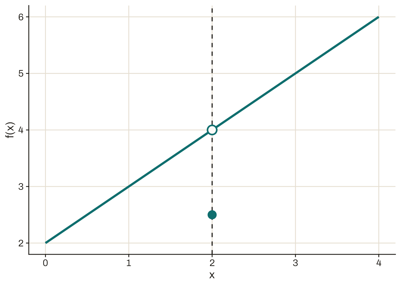
From the graph, it sure looks like 4 is the limit as x approaches 2. We can also get there with the properties from Proposition 2.3. The “trick” to get started is a fact you might remember from algebra: a^2 - b^2 = (a + b) (a - b) for any pair of real numbers a and b. Applying that to the numerator of f(x) (at x \neq 2), we have \begin{alignedat}{2} \lim_{x \to 2} f(x) &= \lim_{x \to 2} \frac{x^2 - 4}{x - 2} \\ &= \lim_{x \to 2} \frac{(x + 2) (x - 2)}{x - 2} &\quad& \text{($a^2 - b^2$ identity)} \\ &= \lim_{x \to 2} [x + 2] && \text{(Cancellation of terms)} \\ &= \lim_{x \to 2} x + \lim_{x \to 2} 2 && \text{(Addition property)} \\ &= 2 + 2 && \text{(Local identity; local constant)} \\ &= 4. \end{alignedat}

Exercise 2.2 (Limit of a fraction) Consider the function f : [0, 5] \to \mathbb{R} defined by \begin{aligned} f(x) = \begin{cases} \frac{2x^2 - x - 15}{x - 3} & \text{if $x \neq 3,$} \\ 10 & \text{if $x = 3$.} \end{cases} \end{aligned} Graph the function, then use the properties of limits to calculate its limit as x \to 3.

Answer

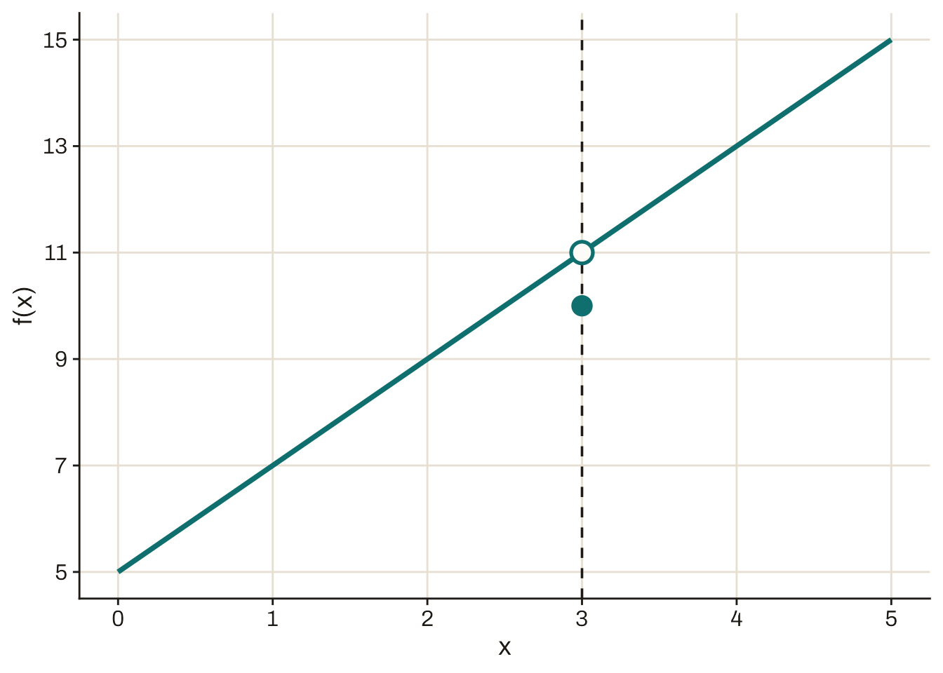
As in the example in the text, we begin with some algebra on the numerator: 2x^2 - x - 15 = (2x + 5) (x - 3). From there we have \begin{alignedat}{2} \lim_{x \to 3} f(x) &= \lim_{x \to 3} \frac{2x^2 - x - 15}{x - 3} \\ &= \lim_{x \to 3} \frac{(2x + 5) (x - 3)}{x - 3} &\quad& \text{(Substitution)} \\ &= \lim_{x \to 3} [2x + 5] && \text{(Cancellation of terms)} \\ &= \lim_{x \to 3} [2x] + \lim_{x \to 3} 5 && \text{(Addition property)} \\ &= \left(\lim_{x \to 3} 2\right) \left(\lim_{x \to 3} x\right) + 5 && \text{(Multiplication property; local constant)} \\ &= 2 \cdot 3 + 5 && \text{(Local constant; local identity)} \\ &= 11. \end{alignedat}

Exercise 2.3 (Limit of a linear function) A linear function is a function f : X \to \mathbb{R} defined by f(x) = \alpha + \beta x, where the domain X consists of real numbers and where (intercept) \alpha and (slope) \beta are constant real numbers. Using the properties of limits, show that for any domain point c \in X, \lim_{x \to c} [\alpha + \beta x] = \alpha + \beta c.

Answer

\begin{alignedat}{2} \lim_{x \to c} [\alpha + \beta x] &= \lim_{x \to c} \alpha + \lim_{x \to c} [\beta x] &\quad& \text{(Addition property)} \\ &= \alpha + \left(\lim_{x \to c} \beta\right) \cdot \left(\lim_{x \to c} x\right) && \text{(Local constant; multiplication property)} \\ &= \alpha + \beta c. && \text{(Local constant; local identity)} \end{alignedat}

The limit you found in Exercise 2.3 is actually a special case of the limit of a polynomial. A polynomial is a sum of terms of the form c_k x^k, where each power k is a non-negative integer, with a corresponding coefficient c_k that is a constant real number. For example, the quadratic function f(x) = 3 x^2 - 7 x + 4 is a polynomial: \begin{aligned} f(x) &= 3 x^2 - 7 x + 4 \\ &= \underbrace{3}_{c_2} \cdot x^2 + \underbrace{(-7)}_{c_1} \cdot \underbrace{x^1}_{=x} + \underbrace{4}_{c_0} \cdot \underbrace{x^0}_{=1}. \end{aligned} Using summation notation, we can say that a polynomial is a function of the form \begin{aligned} f(x) = \sum_{k=0}^n c_k x^k = c_0 + c_1 x + c_2 x^2 + \cdots + c_n x^n. \end{aligned} A linear function is the special case of a polynomial where n = 1, c_0 is the intercept \alpha, and c_1 is the slope \beta.

Summation notation

Don’t remember what \sum means? Don’t panic! It’s the summation symbol, which we use when we’re adding many things together. For example, think about summing up the square of every number from 1 to 39. We could write that as 1^2 + 2^2 + \cdots + 38^2 + 39^2. A shorter way to write that, with the added advantage of leaving absolutely no ambiguity about precisely what we’re summing up, would be with the summation symbol: \sum_{n=1}^{39} n^2. What this means is: for each integer value of n going from 1 to 39, calculate n^2, and then add up all the results.

More generally, the notation \sum_{i=m}^n x_i stands for the sum x_m + x_{m+1} + \cdots + x_{n-1} + x_n. Or in words: for each integer value of i going from m to n, calculate some-function-of-i-that-we’re-denoting-x_i, and then add up all the results.

We often use i to denote the index being summed over, but not always. For example, in the definition of a polynomial, I feel like x^i looks weird in a way that x^k doesn’t, so I use k as the index for the summation instead.

Any polynomial function f(x) has the property you showed for linear functions in Exercise 2.3, namely that \lim_{x \to d} f(x) = f(d). (I’m now using d instead of c to denote the point at which the limit is being taken, simply to avoid confusion with the polynomial coefficients c_0, \ldots, c_n.) To see why, think about how each term of a polynomial is constructed. The k’th term is the product of one constant and k identities, c_k x^k = c_k \cdot \underbrace{x \cdot x \cdots \cdot x}_{k \text{ times}}, so the multiplication rule, the local constant property, and the local identity property tell us that \lim_{x \to d} c_k x^k = \left(\lim_{x \to d} c_k\right) \cdot \underbrace{\left(\lim_{x \to d} x\right) \cdot \left(\lim_{x \to d} x\right) \cdots \cdot \left(\lim_{x \to d} x\right)}_{k \text{ times}} = c_k d^k. A polynomial function is the sum of each of these pieces from k = 0 up to k = n, so we can take the limit by using the addition rule n times: \begin{aligned} \lim_{x \to d} f(x) &= \lim_{x \to d} \left[c_0 + c_1 x + c_2 x^2 + \cdots + c_n x^n\right] \\ &= \lim_{x \to d} c_0 + \lim_{x \to d} [c_1 x] + \lim_{x \to d} [c_2 x^2] + \cdots + \lim_{x \to d} [c_n x^n] \\ &= c_0 + c_1 d + c_2 d^2 + \cdots + c_n d^n \\ &= f(d). \end{aligned} As we’ll see soon, this means every polynomial is continuous throughout its domain.

2.2.3 Left- and right-hand limits

The next graph, which is loosely based on Figure 2.1, illustrates a problem scenario for “the” limit. If you approach c = 0 from the left (values of x just under c = 0), the limit appears to be 60. But if you approach from the right instead (values of x just above c = 0), it appears to be 50. So what is the limit?

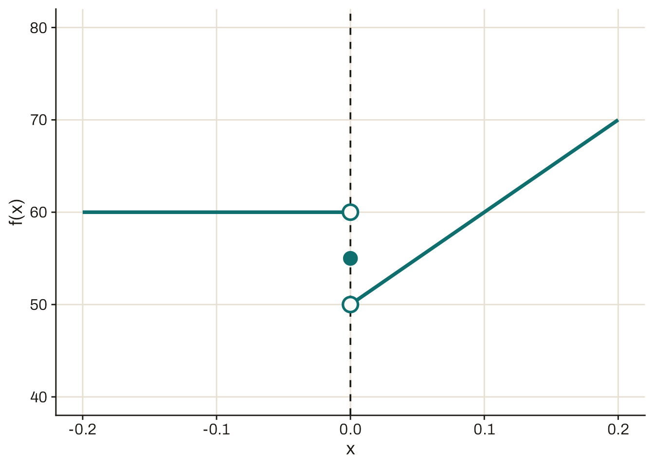
Figure 2.6: A function with differing left- and right-hand limits.

Indeed, the function graphed here is one whose left-hand limit and right-hand limit differ as x approaches 0.

Definition 2.2 (Left- and right-hand limits, informal) Consider a function f : X \to Y, where X \subseteq \mathbb{R} and Y \subseteq \mathbb{R}. Let c be a point in the domain of f, i.e., c \in X.

We say that a number y is the left-hand limit of f(x) as x approaches c, denoted \lim_{x \to c^-} f(x) = y, if f(x) is very close to y whenever x is just below (but not exactly equal to) c.

Similarly, we say that y is the right-hand limit of f(x) as x approaches c, denoted \lim_{x \to c^+} f(x) = y, if f(x) is very close to y whenever x is just above (but not exactly equal to) c.

So for the function graphed in Figure 2.6, we would say the left-hand limit as x approaches 0 is 60, whereas the right-hand limit as x approaches 0 is 50. Or in mathematical notation, \begin{aligned} \lim_{x \to 0^-} f(x) &= 60; \\ \lim_{x \to 0^+} f(x) &= 50. \end{aligned}

What, then, is the overall (not one-sided) limit of f(x) as x approaches 0? It’s not 60, as f(x) only gets close to 60 from the left, not the right. By parallel reasoning, it’s also not 50, which f(x) only gets close to from the right. But it can’t be any other number either, as 50 and 60 are the only numbers it gets close to at all. In fact, the limit of the function as x approaches 0 does not exist.

Anytime the left- and right-hand limits differ at a point, the function has no overall limit at that point. Conversely, if the function does have a limit at a point, the left- and right-hand limits both coincide with the overall limit.

Proposition 2.4 (One-sided limits and the overall limit) If \lim_{x \to c^-} f(x) = y and \lim_{x \to c^+} f(x) = y, then \lim_{x \to c} f(x) = y.

If \lim_{x \to c^-} f(x) \neq \lim_{x \to c^+} f(x), or either of these does not exist, then \lim_{x \to c} f(x) does not exist. Equivalently, if \lim_{x \to c} f(x) = y, then \lim_{x \to c^-} f(x) = \lim_{x \to c^+} f(x) = y.

You’ll notice from the statement of Proposition 2.4 that the one-sided limits may also fail to exist. This is possible in principle, though it’s not common for the functions you’ll run into in political science coursework.

Optional: Examples of one-sided limit non-existence

One way for the one-sided limit not to exist is for the function to oscillate more and more quickly as you approach the point. For example, consider the function f : [0, 1] \to [-1, 1] defined by f(x) = \begin{cases} 0 & \text{if $x = 0$}, \\ \sin (1/x) & \text{if $x > 0$.} \end{cases}

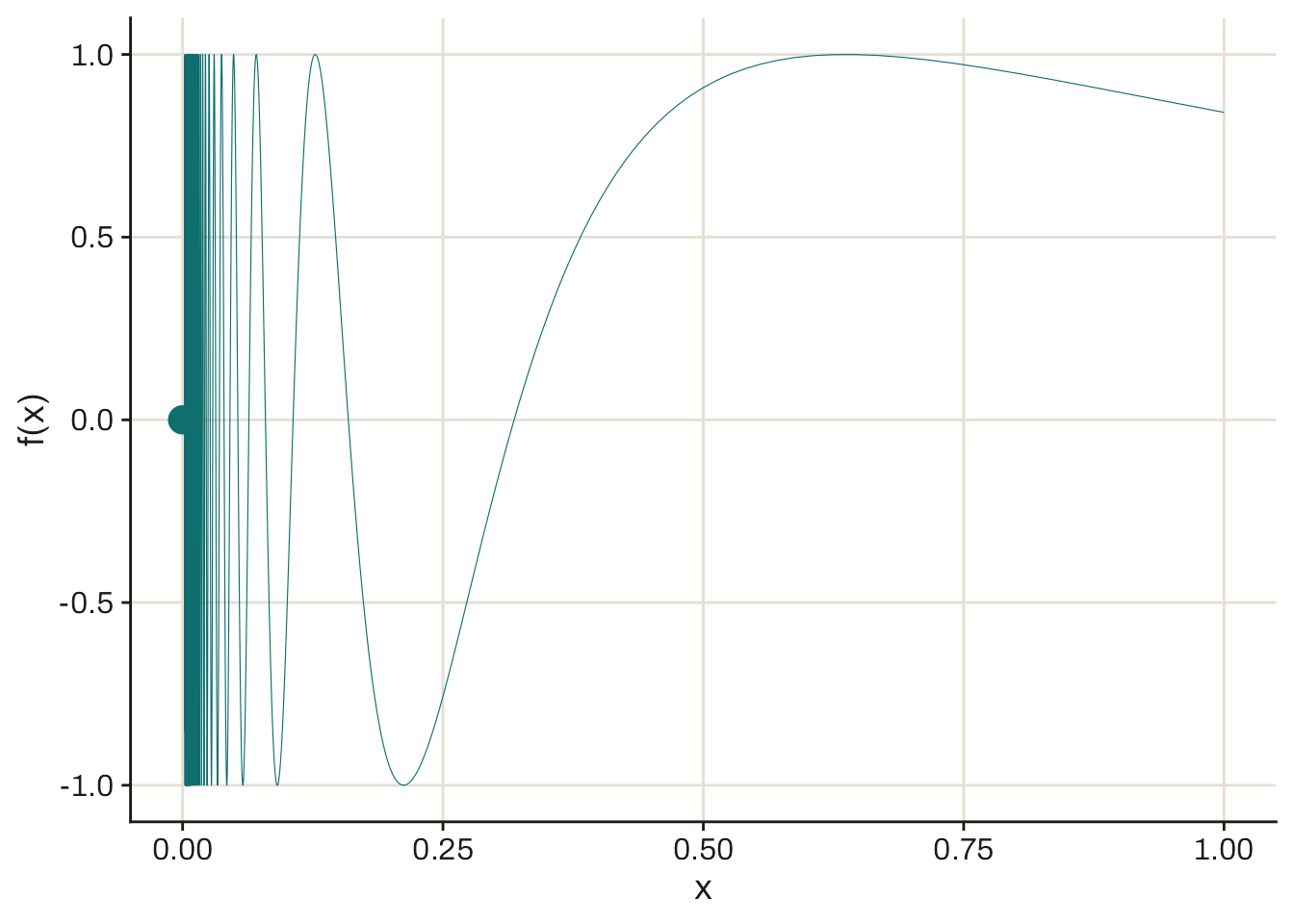
As x gets closer and closer to 0 from above, the function keeps oscillating between -1 and 1 at an increasingly fast rate. Hence, there is no single point that f(x) gets closer and closer to, so \lim_{x \to 0^+} f(x) does not exist.

The other most common way for a one-sided limit not to exist is for the function to be defined in an off-kilter or adversarial way. This is a mode of reasoning that comes up often in pure mathematics, but whose practical applications in political science are limited at most. One famous example is the Dirichlet function, f : \mathbb{R} \to \{0, 1\} defined by f(x) = \begin{cases} 0 & \text{if $x$ is irrational}, \\ 1 & \text{if $x$ is rational}. \end{cases} So we have f(3.14159) = 1, but f(\pi) = 0. Because any interval of real numbers, no matter how small, contains both rational and irrational numbers—a property known as density in the reals—the one-sided limits of the Dirichlet function fail to exist for all domain points c \in \mathbb{R}. That is an interesting fact for mathematicians, but not one that you will run into very often as a political scientist.

One more helpful fact about one-sided limits: all of the properties listed in Section 2.2.2 carry over to them. For example, \lim_{x \to c^-} [f(x) + g(x)] = \lim_{x \to c^-} f(x) + \lim_{x \to c^-} g(x), provided that both of the underlying one-sided limits exist.

Exercise 2.4 (One-sided limits)

Find \lim_{x \to 2^-} [x^2 - 1].
Find \lim_{x \to 2^+} [-2x + 7].
Letting f(x) be defined as in Exercise 2.1, confirm that \lim_{x \to 2} f(x) = 3.

Answer

Applying the standard properties of limits: \begin{aligned} \lim_{x \to 2^-} [x^2 - 1] &= \lim_{x \to 2^-} [x^2] - \lim_{x \to 2^-} 1 \\ &= \lim_{x \to 2^-} [x \cdot x] - 1 \\ &= \left(\lim_{x \to 2^-} x\right) \cdot \left(\lim_{x \to 2^-} x\right) - 1 \\ &= 2 \cdot 2 - 1 \\ &= 3. \end{aligned}
This is a linear function, so your logic from Exercise 2.3 carries over here: \lim_{x \to 2^+} [-2x + 7] = -2 \cdot 2 + 7 = 3.
We have \lim_{x \to 2^-} f(x) = \lim_{x \to 2^-} [x^2 - 1] = 3 = \lim_{x \to 2^+} [-2x + 7] = \lim_{x \to 2^+} f(x), and thus \lim_{x \to 2} f(x) = 3 by Proposition 2.4.

2.3 Continuity

You might notice a pattern in the graphs throughout Section 2.2. At the points in the domain where the value of the function is not equal to its left- or right-hand limit, the graph of the function appears to “jump.” In mathematical terms, we’d say these jumps are points of discontinuity. By contrast, in the parts of the domain where there are no such jumps, the function is continuous.

Definition 2.3 (Continuity at a point) We say that a function f : X \to Y is continuous at the point c \in X if its limit exists at that point and is equal to the value of the function: \lim_{x \to c} f(x) = f(c).

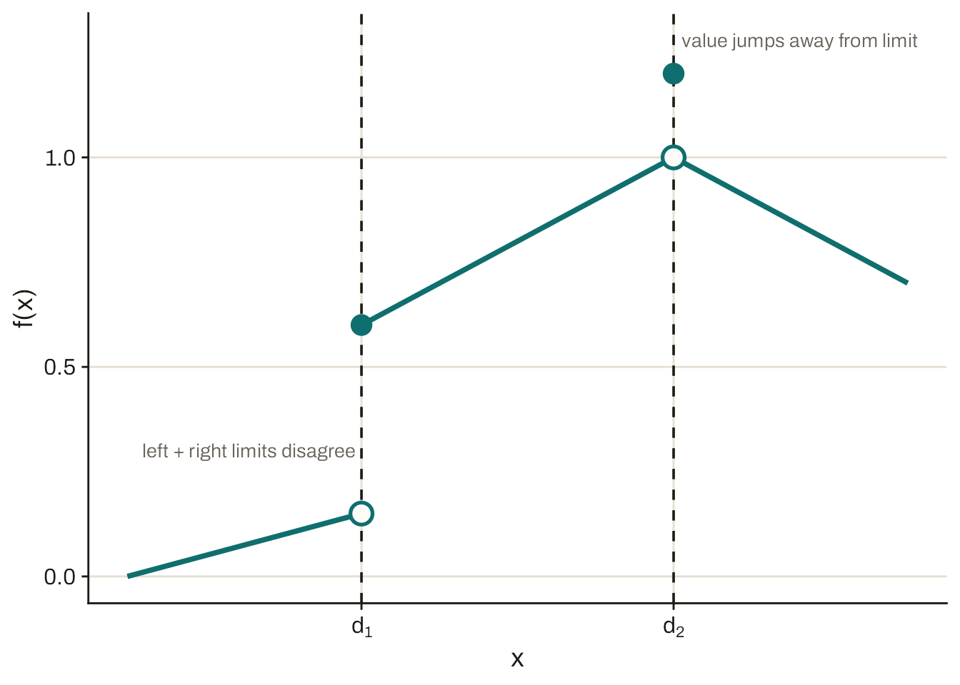
For most functions you’d deal with in practice, you can tell where the function is continuous and where it is not by looking at the graph. You may (or may not) remember past teachers using the heuristic: if you can draw the graph of the function without lifting your pen off the paper, it’s continuous. More to the point, anywhere the left- and right-hand limits do not agree, the function is discontinuous. It is also discontinuous at any point where the limits agree but the function value itself “jumps.” At all other points, the function is continuous. Figure 2.7 illustrates both types of discontinuity.

Figure 2.7: The function is discontinuous at d_1 and d_2, and continuous at all other points.

When a function is continuous at every point in its domain, we call it a continuous function.

Definition 2.4 (Continuous function) We say that a function f : X \to Y is continuous if it is continuous at every point in its domain, X.

When a function f is continuous, every point close to c on the domain has a function value close to f(c). If you think about it this way, you can see why the function illustrated in Figure 2.7 is not continuous. Even at values of x really really close to d_2, there’s going to be a substantial gap between the function values f(x) and f(d_2).

Lots of common functions are continuous. Here are just a few examples of functions you’re likely to run into that are continuous. Except where I note otherwise, each of the functions f : X \to \mathbb{R} below is continuous on any subset of the real numbers, X \subseteq \mathbb{R}.

Identity function: The function f(x) = x is continuous.
Absolute value function: The function f(x) = |x|, or equivalently f(x) = \begin{cases}-x & \text{if $x < 0$},\\x & \text{if $x \geq 0$,}\end{cases} is continuous.
Linear functions: Any function of the form f(x) = a + b x, where a and b are real numbers, is continuous.
Polynomials: Any polynomial is continuous.
Constant multiples of continuous functions: Any function of the form f(x) = c g(x), where c is a real number and g is continuous, is continuous.
Sums and products of continuous functions: Any function of the form f(x) = g(x) + h(x) or f(x) = g(x) h(x), where g and h are continuous, is continuous.
Division by a continuous function: Any function of the form f(x) = 1 / g(x), where g is continuous and g(x) \neq 0 for all x \in X, is continuous.
Compositions of continuous functions: If g and h are continuous, then their composition (Definition 1.11), f(x) = g(h(x)), is continuous.

Exercise 2.5 (Continuous functions) Show that the function f : \mathbb{R} \to \mathbb{R} defined by f(x) = \left| \frac{-7 x^3 - 4 x^2 + x - 37}{x^2 + 10} \right| is continuous.

Answer

First, observe that f is a composite function. We may write f(x) = g(h(x)), where g(x) = |x| and h(x) = \frac{-7 x^3 - 4 x^2 + x - 37}{x^2 + 10}. g is the absolute value function and is therefore continuous. h is a ratio of polynomials, and its denominator is never zero because x^2 + 10 \geq 10 > 0. Therefore, h is continuous as well. Then, because f is the composition of two continuous functions, it is continuous.

Two more classes of continuous functions about which we’ll have more to say in just a second:

Exponential functions: Any function of the form f(x) = a^x, where a > 0, is continuous.
Logarithmic functions: Any function of the form f(x) = \log_b x, where b > 0 and b \neq 1, is continuous on any domain consisting of positive numbers, X \subseteq (0, \infty).

To the extent that it’s sensible to have warm feelings about mathematical objects (don’t judge), we tend to “like” continuous functions. Continuous functions tend to have nice properties, like ensuring the existence of solutions to certain types of problems we might want to solve. The phrase “If f is continuous…” will come up repeatedly once we get into calculus and optimization.

In the meantime, here’s a simpler upshot of continuity. Consider a function with a domain of X, and suppose that domain includes the interval [a, b]. As we travel from left to right across that interval, the value of the function goes from f(a) to f(b). And as you’ll see if you try to draw any continuous function—keeping in mind the “it’s continuous if and only if you can draw its graph without lifting the pen off the page” rule—along that path, it ends up touching every single value between f(a) and f(b). This is a famous result called the intermediate value theorem.

Theorem 2.1 (Intermediate value theorem) Consider a continuous function f : X \to Y, where X \subseteq \mathbb{R} and Y \subseteq \mathbb{R}. Consider any interval in the domain, [a, b] \subseteq X. For any real number y that satisfies f(a) < y < f(b) \quad \text{or} \quad f(b) < y < f(a), there is a domain point c \in (a, b) such that f(c) = y.

As you saw in the discussion of non-existent limits above, one frustrating thing about “higher” math is that some problems turn out not to have a solution. The intermediate value theorem often proves useful to show that a problem has a solution, even if it doesn’t tell us what that solution is.

Exercise 2.6 (Intermediate value theorem) Consider the function f : [0, 10] \to \mathbb{R} defined by f(x) = x^4 + x^3 + x^2 + x + 1. Using the intermediate value theorem, show that there is a value c \in [0, 10] for which f(c) = 1{,}017. You do not need to find the exact value of c, just show that a solution exists.

Answer

Notice that \begin{aligned} f(0) &= 0^4 + 0^3 + 0^2 + 0 + 1 \\ &= 1, \\ f(10) &= 10^4 + 10^3 + 10^2 + 10 + 1 \\ &= 10{,}000 + 1{,}000 + 100 + 10 + 1 \\ &= 11{,}111. \end{aligned} f is a polynomial and therefore is continuous. Because f(0) < 1{,}017 < f(10), the intermediate value theorem implies that there is a c \in (0, 10) that solves f(c) = 1{,}017.

A final note on continuity. I already mentioned that continuity will be useful as we move into the calculus backdrop for statistics. But going back to Figure 2.1, as you get even deeper into the stats sequence next semester, you’ll see that discontinuity is useful to establish certain causal inferences. So you’ll need to have your head wrapped around the mathematical meanings of continuity and discontinuity to understand the underpinnings of that technique too.

2.4 Exponential and logarithmic functions

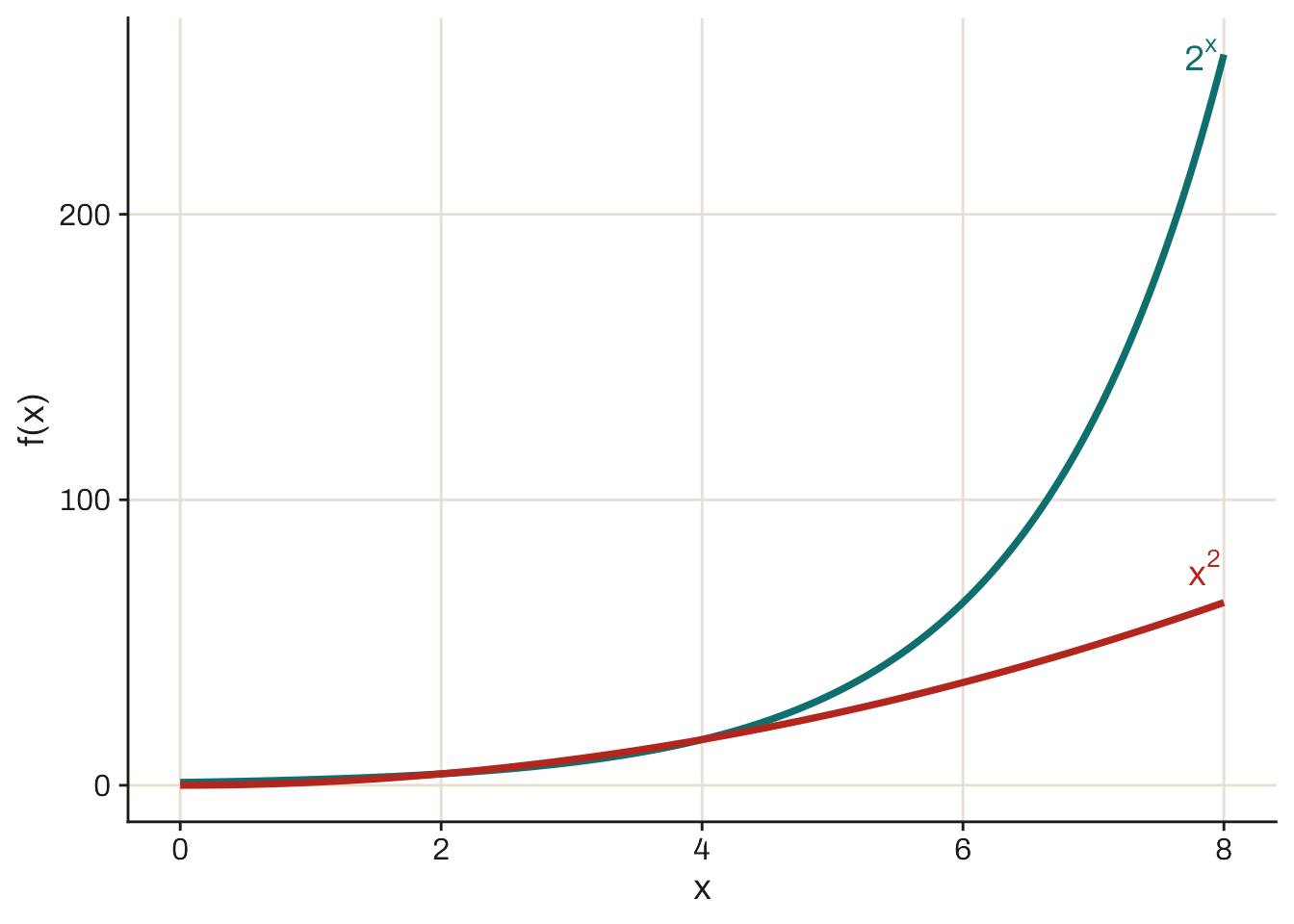
A function in the form f(x) = x^b, where the variable x is raised to the power of some fixed constant b, is probably familiar to you. In fact, when b is a non-negative integer, a function in this form is a simple example of a polynomial. An exponential function has a similar form, but now with the variable as the power: f(x) = b^x. Exponential functions with bases b > 1 increase really quickly, hence the term “exponential growth.”

Figure 2.8: The exponential function 2^x compared to the polynomial x^2.

2.4.1 Logarithms

A logarithm is the reverse of an exponent. It is how we “solve for x” in an equation like b^x = a, where a > 0 and b > 0 are known constants.

Definition 2.5 (Logarithm) For any positive number a and any positive number b \neq 1, we say that x = \log_b a (pronounced “x is the logarithm, base b, of a”) if and only if b^x = a.

Here are a few examples of logarithms in action.

Because 2^3 = 2 \times 2 \times 2 = 8, we have \log_2 8 = 3. In words, 3 is the base-2 logarithm of 8.
Because 10^{-2} = \frac{1}{10^2} = \frac{1}{100} = 0.01, we have \log_{10} 0.01 = -2. In words, -2 is the base-10 logarithm of 0.01.
Because 64^{1/2} = \sqrt{64} = 8, we have \log_{64} 8 = 1/2. In words, 1/2 is the base-64 logarithm of 8.

Exercise 2.7 (Logarithms in practice) Imagine an incumbent politician who faces a probability p \in (0, 1) of re-election each term she serves. The probability that she will serve exactly t more terms is \begin{aligned} \Pr(\text{win $t$ times}) \cdot \Pr(\text{lose the $t+1$'th}) = \underbrace{p \cdot p \cdots \cdot p}_{t \text{ times}} \cdot (1 - p) = p^t (1 - p). \end{aligned} Suppose you wanted to calculate the largest number of additional terms that the politician would have a probability q or greater of serving. In other words, you want to find the greatest value of t such that p^t (1 - p) \geq q. What logarithm should you calculate?

Answer

Momentarily ignoring the fact that the term length must be a whole number, let’s find the t at which the probability of serving t more terms is exactly q. We want to solve for t in p^t (1 - p) = q, which is equivalent to solving for t in p^t = \frac{q}{1 - p}. By the definition of a logarithm, Definition 2.5, this means t = \log_p \frac{q}{1 - p}. If t happens to be a whole number, this is our answer; otherwise, we need to round down. (In numerical programming terms, we want to take the “floor” of \log_p \frac{q}{1 - p}.)

2.4.2 Properties of exponents and logarithms

Logarithms come up surprisingly often in mathematical writing and in statistical programming, even in contexts where we’re not solving equations of the form a^x = b. They’re useful because of their helpful properties, some of which we’ll now review.

Logarithm of a product. You might remember that b^{y + z} = b^y \times b^z. As an example to make this more concrete, think about 2^5: 2^5 = 2^{2 + 3} = \underbrace{2 \times 2}_{2^2} \times \underbrace{2 \times 2 \times 2}_{2^3} = 2^2 \times 2^3.

This fact about exponents is the basis for an extremely helpful property of logarithms: the logarithm of a product is the sum of the logarithms.

Proposition 2.5 (Logarithm of a product) For any positive numbers y and z and any positive number b \neq 1, \log_b (y \times z) = \log_b y + \log_b z.

Proof. By the definition of the logarithm and the property of products of exponents, b^{\log_b y + \log_b z} = b^{\log_b y} \times b^{\log_b z} = y \times z. Therefore, again by the definition of the logarithm, \log_b (y \times z) = \log_b y + \log_b z.

This property of logarithms is highly useful in both statistical computing and in calculus. In the statistical context, suppose you need to calculate the probability of some very large number of independent events, resulting in a calculation that looks like p_1 \times p_2 \times \cdots \times p_N, where N is some huge number. (For one thing, calculations like this are central to maximum likelihood estimation.) It turns out that computers are not so good at multiplying a lot of very small numbers together. At a certain point, as in the following example, the computer can’t distinguish the product from 0.

# Randomly sample a bunch of numbers each close to 1/100
size <- 500
tiny_numbers <- runif(size, min = 0.009, max = 0.011)

# Double check that every number is positive
all(tiny_numbers > 0)

[1] TRUE

# prod() to multiply all numbers in a vector together
prod(tiny_numbers)

[1] 0

# Not just visual rounding: R thinks the product is zero!
prod(tiny_numbers) == 0

[1] TRUE

The standard arithmetic algorithms on a computer aren’t designed to represent numbers as small as the product of these 500 tiny probabilities. But we can still calculate a precise mathematical expression for the product—we just need to convert our probability-multiplication problem into a logarithm-addition problem. Using Proposition 2.5, we know that for any positive base b \neq 1, \log_b (p_1 \times p_2 \times \cdots \times p_N) = \log_b p_1 + \log_b p_2 + \cdots + \log_b p_N. Let’s use a base of b = 10, since then we can interpret our result in terms of decimal places.

# Convert each number to its base-10 log
logged_numbers <- log(tiny_numbers, base = 10)

# sum() to add all numbers in a vector together
sum(logged_numbers)

[1] -1001.661

Now we have a much more accurate calculation: the product of the 500 small numbers we randomly drew is 10^{-1001.661}.

Logarithm of a power. Again thinking about exponents, you might remember that (b^y)^z = b^{y \times z}. For example, think about 5^6: 5^6 = 5^{3 \times 2} = \underbrace{5 \times 5 \times 5}_{5^3} \times \underbrace{5 \times 5 \times 5}_{5^3} = (5^3)^2. This property of exponents delivers us another helpful property of logarithms: the log of y to the z’th power is z times the log of y. Or, as I think of it, logarithms turn powers into coefficients.

Proposition 2.6 (Logarithm of a power) For any positive number y, any number z, and any positive base b \neq 1, \log_b (y^z) = z \log_b y.

Proof. By the definition of the logarithm and the property of powers of exponents, b^{z \log_b y} = (b^{\log_b y})^z = y^z. Therefore, again by the definition of the logarithm, \log_b (y^z) = z \log_b y.

Logarithm of a ratio. We saw in Proposition 2.5 that logarithms turn multiplication problems into addition problems. For similar reasons, they turn division problems into subtraction problems.

Proposition 2.7 (Logarithm of a ratio) For any positive number y, any positive number z, and any positive base b \neq 1, \log_b \left(\frac{y}{z}\right) = \log_b y - \log_b z.

You’ve already got the tools you need to prove this one yourself, so I’m leaving the proof as an exercise for you.

Exercise 2.8 Prove Proposition 2.7. (Hint: use both of the two previous properties of logarithms, Proposition 2.5 and Proposition 2.6.)

Answer

The ratio \frac{y}{z} is equivalent to the product y \times z^{-1}. Therefore, Proposition 2.5 implies \log_b \left(\frac{y}{z}\right) = \log_b (y \times z^{-1}) = \log_b y + \log_b (z^{-1}). Furthermore, Proposition 2.6 gives us \log_b (z^{-1}) = - \log_b z. We conclude that \log_b \left(\frac{y}{z}\right) = \log_b y + \log_b (z^{-1}) = \log_b y - \log_b z.

Logarithm of 1. The number 1 is special. Perhaps you recall the mathematical rule that b^0 = 1 for any positive number b. It follows immediately that the logarithm of 1 is always 0, regardless of which base we are working with.

Proposition 2.8 (Logarithm of 1) For any positive base b \neq 1, \log_b 1 = 0.

Let’s go back to this rule that b^0 = 1 for any positive number b. The mathematical expression b^0 is confusing. We typically think of b^x as meaning “multiply b together x times.” How can we multiply b together 0 times? What does that even mean?

I’m sure someone out there has a deep explanation of why it makes sense for b^0 to equal 1. But I’m a mathematical pragmatist. What I know is that our rule that b^{x + y} = b^x \times b^y would completely break down if b^0 had any value other than 1. For example, imagine instead that we had b^0 = 42 for some base b. Well, then, our usual rule about exponents of sums would give us b = b^1 = b^{0 + 1} = b^0 \times b^1 = 42 b. That can’t be right! The only sensible way forward is to assume b^0 = 1. I don’t lose any sleep over not having some kind of physical or visual intuition why this is the case, because I know that it’s the only way to handle powers of 0 that doesn’t cause other important things to break.

Sometimes you’ll run into things like this in mathematics. It’s different for everyone. Some people get hung up on the “imaginary” number i = \sqrt{-1}, which I’m happy to tell you basically never comes up in the work political scientists do. Others get hung up on the idea of spaces with more than 3 dimensions, which very much do come up in the work we do. Heck, I know people who are skeptical of the idea of negative numbers because they can’t visualize them.

Whenever I run into one of these things that I can’t directly visualize or comprehend with a physical analogy, I instead try to think about its role in the mathematical system I’m working with. I can’t “see” why b^0 = 1, but I know that it ensures b^{x + y} = b^x \times b^y. I can’t “picture” the imaginary number i, but I know that it lets us solve algebraic equations like x^2 + 4 = 0. I definitely can’t “visualize” a linear function through 631-dimensional space, yet while I was writing these notes my computer was estimating a regression model with 631 parameters. Don’t feel like you have to be able to picture every mathematical rule or object—it’s enough just to understand how it helps you solve a particular problem.

Base changes and the natural logarithm. Suppose we know that the base-2 logarithm of 16 is 4, i.e., \log_2 16 = 4. What, if anything, does this tell us about the base-8 logarithm of 16?

It turns out that there’s a pretty handy formula to change a logarithm from one base to another. To change the base-b logarithm of y to a base-c logarithm, we just rescale it by the base-b logarithm of c.

Proposition 2.9 (Logarithm base changes) For any positive number y and any positive bases b \neq 1 and c \neq 1, \log_c y = \frac{\log_b y}{\log_b c}.

Proof. Using the definition of a logarithm twice and the properties of exponents once, we have y = c^{\log_c y} = (b^{\log_b c})^{\log_c y} = b^{(\log_b c) \times (\log_c y)}. Therefore, again by the definition of a logarithm, \log_b y = (\log_b c) \times (\log_c y). We obtain the proposition by dividing both sides by \log_b c.

Now we can calculate the base-8 logarithm of 16. Since 2^4 = 16, we know that \log_2 16 = 4. And since 2^3 = 8, we know that \log_2 8 = 3. Therefore, using Proposition 2.9, we have \log_8 16 = \frac{\log_2 16}{\log_2 8} = \frac{4}{3}.

In a sense, the upshot of Proposition 2.9 is that it doesn’t matter what base we use—the value of the logarithm scales up or down with the value of the base, but the shape of the curve is the same regardless, as illustrated in Figure 2.9. So if we’re doing something like logging a variable in a linear regression, our results will be substantively the same regardless of which logarithmic base we use. Since the choice of base doesn’t substantively affect our findings, we should choose whatever base is most convenient for interpretation.

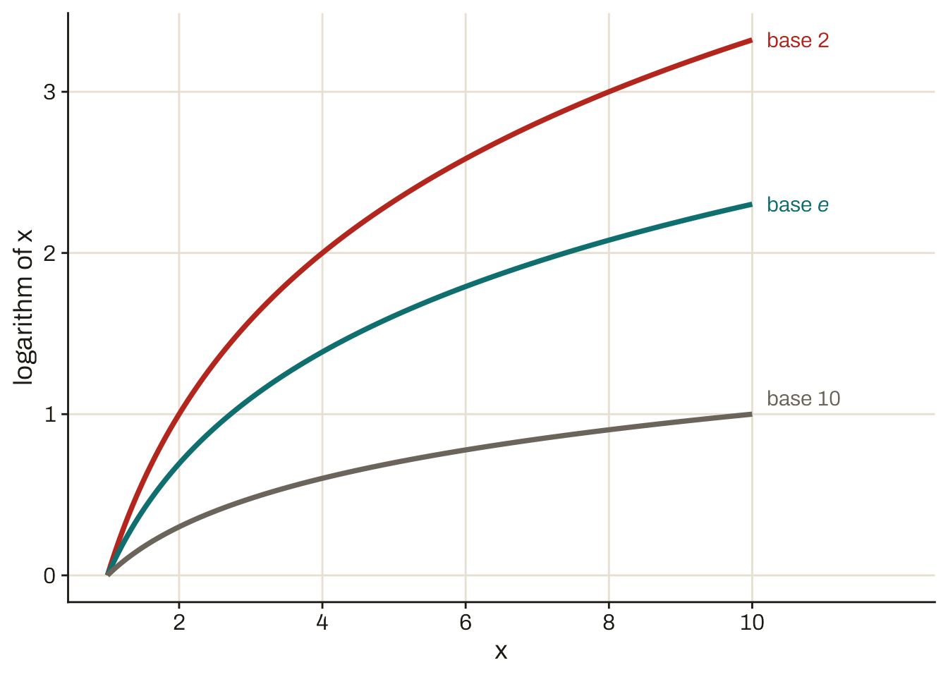
Figure 2.9: Logarithms with different bases

This figure shows three common choices of base for the logarithm. You are probably familiar with the numbers 2 and 10. You might be less familiar with the number e, aka Euler’s number, which is equal to roughly 2.718 and comes up repeatedly in high-end math. This number is important enough that we call the base-e logarithm the natural logarithm. For now, I’m going to ask you to trust me that e is important—you’ll be able to see the reasoning a bit better once we get to calculus.

In these notes, when I write \log y without an explicit base, I mean the natural logarithm of y. Similarly, the log() function in R takes the natural logarithm if you don’t specify a base. If you want to take a base-e exponent in R, use the exp() function.

Proposition 2.9 tells us why it’s mostly harmless to just use the natural logarithm for everything. If for some reason you ever need to convert a natural logarithm to a different base, you can just use the formula \log_b y = \frac{\log y}{\log b}.

log versus ln

In other contexts, including high school math (if my early-2000s experience still holds), people use “ln” to mean the natural logarithm and “log” to mean the base-10 logarithm. ChatGPT tells me that engineers are also fond of this usage. But in political science, economics, and statistics writing, as well as in the overwhelming majority of math textbooks at the college level and beyond, “log” means the natural logarithm.

2.5 (optional) Defining limits formally

To formally define the limit of a function, mathematicians employ what I think of as a challenge-response structure. Suppose I have a function f, and I want to claim that \lim_{x \to c} f(x) = y, i.e., the limit of the function as x approaches the point c in its domain is equal to y.

You challenge me by picking an \epsilon > 0.

Think of this as you saying “I need you to show me that if we are close enough to x = c on the domain of the function, then the value of f(x) is within \epsilon of your claimed limit, y.”
I respond to the challenge by identifying a value \delta > 0. I need to show you that if 0 < |x - c| < \delta, then we have |f(x) - y| < \epsilon.

In words, at any point on the domain whose distance from c is less than \delta (other than c itself), the value of the function is at least as close to my claimed limit as you challenged me to show.

If I can conjure up a valid response to any \epsilon > 0 challenge that you might issue, then my claim about the limit of the function stands. This line of reasoning gives us our formal definition of the limit of a function.

Definition 2.6 (Limit of a function, formal) Let X \subseteq \mathbb{R} be an open interval, and consider the function f: X \to \mathbb{R}. For a point c \in X, we say that the limit as x approaches c equals y, denoted \lim_{x \to c} f(x) = y, if the following condition holds: for any value of \epsilon > 0, there exists a value \delta > 0 such that |f(x) - y| < \epsilon for all x satisfying 0 < |x - c| < \delta.

To make this definition a bit more concrete, let’s practice using the formal definition to show that f(x) \to 1 as x \to 0 for the function illustrated in Figure 2.2.

We’ll start by considering any “challenge” \epsilon > 0. This is akin to someone telling us: you need to show that if x is close enough to 0, then f(x) is within \epsilon of the claimed limit, namely 1. Because we want to show that we can meet any such challenge, we are not going to put a specific value on \epsilon. Instead, we’ll show that for an arbitrary value of \epsilon > 0—a value that we know nothing about, other than the fact that it’s a positive number—we can find a \delta that satisfies the challenge.

Our response to the challenge will be \delta = \epsilon / 2. We need to show that if 0 < |x - 0| < \delta, then |f(x) - 1| < \epsilon. Equivalently, we need to show that if x \in (-\delta, 0) \cup (0, \delta), then -\epsilon < f(x) - 1 < \epsilon. We’ll do this in two parts.

For all x \in (-\delta, 0), we have f(x) = 1 + 2x > 1 + 2(-\delta) = 1 + 2\left(-\frac{\epsilon}{2}\right) = 1 - \epsilon and f(x) = 1 + 2x < 1 + 2(0) = 1. Therefore, for all such x, we have -\epsilon < f(x) - 1 < 0 < \epsilon, as required.
For all x \in (0, \delta), we have f(x) = 1 + 2x > 1 + 2(0) = 1 and f(x) = 1 + 2x < 1 + 2\delta = 1 + 2\left(\frac{\epsilon}{2}\right) = 1 + \epsilon. Therefore, for all such x, we have -\epsilon < 0 < f(x) - 1 < \epsilon, as required.

We have shown that for any challenge \epsilon > 0 to our claim that \lim_{x \to 0} f(x) = 1, we have a valid response, namely \delta = \epsilon/2. Therefore, we have proved that \lim_{x \to 0} f(x) = 1.

The restriction to open interval domains

Definition 2.6 states the formal definition of the limit only for functions whose domain is an open interval. Under this stipulation, the domain X must take one of the four following forms:

X is the whole real line, X = \mathbb{R}.
X is the set of numbers strictly greater than some real number a, X = \{x \in \mathbb{R} \mid x > a\} = (a, \infty).
X is the set of numbers strictly less than some real number b, X = \{x \in \mathbb{R} \mid x < b\} = (-\infty, b).
X is the set of numbers strictly greater than some real number a and strictly less than some real number b, X = \{x \in \mathbb{R} \mid a < x < b\} = (a, b).

This restriction ensures that for any c \in X, it is possible to find a \delta small enough that (c - \delta, c + \delta) \subseteq X, and thus the value of f(x) is well-defined for all x \in (c - \delta, c + \delta).

The formal definition of a limit for a function with a different type of domain has a similar challenge-response structure. It just involves even more annoying technical difficulties, and we are already far enough into the realm of annoying technical difficulty here that I thought it’d be best to focus on the least-worst case.

2.6 Concept review

Limit of a function: The limit of f(x) as x approaches c, denoted \lim_{x \to c} f(x), is the value that f(x) gets closer and closer to as x gets closer and closer to c without reaching it. A function may not have a limit at a particular point.
Continuity: A function is continuous at a point c in its domain if the value of the function there is the same as its limit: f(c) = \lim_{x \to c} f(x). If a function is continuous at every point in its domain, we call it a continuous function.
Linear function: A function of the form f(x) = \alpha + \beta x, where \alpha and \beta are constant real numbers.
Polynomial: A function of the form f(x) = c_0 + c_1 x + \cdots + c_n x^n = \sum_{k=0}^n c_k x^k, where each coefficient c_i is a constant real number.
Summation: A concise way to denote adding up many terms. The notation \sum_{i=1}^n x_i is shorthand for x_1 + x_2 + \cdots + x_n.
Left-hand limit: The left-hand limit of f(x) as x approaches c, \lim_{x \to c^-} f(x), also called the limit of f(x) as x approaches c from below, is the value that f(x) gets closer and closer to as x takes values just below c without reaching it.
Right-hand limit: The right-hand limit of f(x) as x approaches c, \lim_{x \to c^+} f(x), also called the limit of f(x) as x approaches c from above, is the value that f(x) gets closer and closer to as x takes values just above c without reaching it.
Intermediate value theorem: If f is continuous and its domain includes the interval [a, b], then for all values y between f(a) and f(b), there is a point c \in (a, b) such that f(c) = y.
Exponential function: A function of the form f(x) = b^x, where b > 0 is a constant.
Logarithm: The reverse of an exponent. In particular, for any numbers a > 0 and b > 0, if b^x = a, then we say that x = \log_b a. In this example, b is called the base of the logarithm. For example, \log_{10} 1000 = 3 because 10^3 = 1000.
Natural logarithm: A logarithm whose base is Euler’s number, e, the mathematical constant equal to roughly 2.718. Whenever you see \log without an explicit base, you can assume it means a natural logarithm.

Continuity: A function is continuous at a point c in its domain if the value of the function there is the same as its limit: f(c) = \lim_{x \to c} f(x). If a function is continuous at every point in its domain, we call it a continuous function.
Exponential function: A function of the form f(x) = b^x, where b > 0 is a constant.
Intermediate value theorem: If f is continuous and its domain includes the interval [a, b], then for all values y between f(a) and f(b), there is a point c \in (a, b) such that f(c) = y.
Left-hand limit: The left-hand limit of f(x) as x approaches c, \lim_{x \to c^-} f(x), also called the limit of f(x) as x approaches c from below, is the value that f(x) gets closer and closer to as x takes values just below c without reaching it.
Limit of a function: The limit of f(x) as x approaches c, denoted \lim_{x \to c} f(x), is the value that f(x) gets closer and closer to as x gets closer and closer to c without reaching it. A function may not have a limit at a particular point.
Linear function: A function of the form f(x) = \alpha + \beta x, where \alpha and \beta are constant real numbers.
Logarithm: The reverse of an exponent. In particular, for any numbers a > 0 and b > 0, if b^x = a, then we say that x = \log_b a. In this example, b is called the base of the logarithm. For example, \log_{10} 1000 = 3 because 10^3 = 1000.
Natural logarithm: A logarithm whose base is Euler’s number, e, the mathematical constant equal to roughly 2.718. Whenever you see \log without an explicit base, you can assume it means a natural logarithm.
Polynomial: A function of the form f(x) = c_0 + c_1 x + \cdots + c_n x^n = \sum_{k=0}^n c_k x^k, where each coefficient c_i is a constant real number.
Right-hand limit: The right-hand limit of f(x) as x approaches c, \lim_{x \to c^+} f(x), also called the limit of f(x) as x approaches c from above, is the value that f(x) gets closer and closer to as x takes values just above c without reaching it.
Summation: A concise way to denote adding up many terms. The notation \sum_{i=1}^n x_i is shorthand for x_1 + x_2 + \cdots + x_n.